
Windspharm Tutorial: Spherical Harmonic Wind Analysis#
This tutorial demonstrates how to use the Skyborn windspharm package for spherical harmonic analysis of atmospheric wind fields. We’ll work with real NetCDF data to calculate vorticity, divergence, streamfunction, velocity potential, and perform Helmholtz decomposition.
What is Spherical Harmonic Wind Analysis?#
Spherical harmonic analysis is a mathematical technique used in meteorology to:
Decompose wind fields into rotational and divergent components
Calculate dynamically important quantities like vorticity and divergence
Smooth and filter atmospheric data
Perform spectral truncation for model applications
The windspharm package provides a convenient Python interface for these calculations.
1. Setup and Data Loading#
First, let’s import the necessary packages and load our wind data:
import numpy as np
import xarray as xr
import pandas as pd
import matplotlib.pyplot as plt
import cartopy.crs as ccrs
import cartopy.feature as cfeature
from cartopy.util import add_cyclic_point
import cmaps
import warnings
warnings.filterwarnings('ignore')

# Import windspharm with xarray interface (primary interface)
from skyborn.windspharm.xarray import VectorWind
# Import additional interfaces for advanced usage
from skyborn.windspharm.standard import VectorWind as StandardVectorWind  # standard interface
from skyborn.windspharm.tools import prep_data, recover_data  # data preparation tools

# Import skyborn plotting utilities
from skyborn.plot import add_equal_axes, curly_vector

# Set up matplotlib for better plots
plt.rcParams['figure.figsize'] = (14, 10)
plt.rcParams['font.size'] = 11
plt.rcParams['axes.titlesize'] = 13
plt.rcParams['axes.labelsize'] = 11
config = {
    "font.family": 'DejaVu Sans',
    "font.size": 15,
    # 'font.style': 'normal',
    'font.weight': 'bold',
    "mathtext.fontset": 'stix',
    "font.serif": ['cmb10'],
    "axes.unicode_minus": False,
    "axes.labelweight": "bold",
    "axes.labelsize": 15,
}
plt.rcParams.update(config)
print("Libraries imported successfully!")
print("cmaps and skyborn.plot utilities loaded!")
Libraries imported successfully!
cmaps and skyborn.plot utilities loaded!
# Setup for saving documentation images
from pathlib import Path

# Define the documentation images directory
notebook_dir = Path.cwd()
if 'notebooks' in str(notebook_dir):
    docs_images_dir = notebook_dir.parent / 'images'
else:
    docs_images_dir = Path('docs/source/images')

docs_images_dir.mkdir(parents=True, exist_ok=True)

def save_gallery_figure(fig, filename, dpi=300):
    """Save figure to documentation gallery with high quality"""
    filepath = docs_images_dir / filename
    fig.savefig(filepath, dpi=dpi, bbox_inches='tight', facecolor='white')
    # print(f"✅ Saved gallery image: {filepath}")
    return filepath
Load Real NetCDF Wind Data#
We’ll load U and V wind components from NetCDF files. These contain monthly mean wind data on a regular latitude-longitude grid:
# Load wind data from NetCDF files
data_path = '../../../src/skyborn/windspharm/examples/example_data/'

# Load datasets
ds_u = xr.open_dataset(data_path + 'uwnd_mean.nc')
ds_v = xr.open_dataset(data_path + 'vwnd_mean.nc')

# Extract wind components as DataArrays
u_wind = ds_u.uwnd
v_wind = ds_v.vwnd

print("Wind data loaded successfully!")
print(f"U wind shape: {u_wind.shape}")
print(f"V wind shape: {v_wind.shape}")
print(f"Coordinate dimensions: {u_wind.dims}")
print(f"\nLatitude range: {u_wind.latitude.min().values:.1f}° to {u_wind.latitude.max().values:.1f}°")
print(f"Longitude range: {u_wind.longitude.min().values:.1f}° to {u_wind.longitude.max().values:.1f}°")
print(f"Time steps: {len(u_wind.time)} months")
Wind data loaded successfully!
U wind shape: (12, 73, 144)
V wind shape: (12, 73, 144)
Coordinate dimensions: ('time', 'latitude', 'longitude')

Latitude range: -90.0° to 90.0°
Longitude range: 0.0° to 357.5°
Time steps: 12 months
Explore the Wind Data#
Let’s examine the structure and properties of our wind data:
# Display data information
print("=== U Wind Component ===")
print(u_wind)
print("\n=== V Wind Component ===")
print(v_wind)

# Check data ranges
print(f"\n=== Data Statistics ===")
print(f"U wind range: {u_wind.min().values:.2f} to {u_wind.max().values:.2f} m/s")
print(f"V wind range: {v_wind.min().values:.2f} to {v_wind.max().values:.2f} m/s")
print(f"Grid resolution: {np.diff(u_wind.latitude.values)[0]:.1f}° latitude, {np.diff(u_wind.longitude.values)[0]:.1f}° longitude")
=== U Wind Component ===
<xarray.DataArray 'uwnd' (time: 12, latitude: 73, longitude: 144)> Size: 505kB
[126144 values with dtype=float32]
Coordinates:
  * time          (time) datetime64[ns] 96B 1970-01-01 1970-02-01 ... 1970-12-01
  * latitude      (latitude) float32 292B 90.0 87.5 85.0 ... -85.0 -87.5 -90.0
  * longitude     (longitude) float32 576B 0.0 2.5 5.0 7.5 ... 352.5 355.0 357.5
    air_pressure  float32 4B ...
Attributes:
    long_name:    Monthly Long Term mean u wind
    units:        m/s
    parent_stat:  Mean
    statistic:    Long Term Mean

=== V Wind Component ===
<xarray.DataArray 'vwnd' (time: 12, latitude: 73, longitude: 144)> Size: 505kB
[126144 values with dtype=float32]
Coordinates:
  * time          (time) datetime64[ns] 96B 1970-01-01 1970-02-01 ... 1970-12-01
  * latitude      (latitude) float32 292B 90.0 87.5 85.0 ... -85.0 -87.5 -90.0
  * longitude     (longitude) float32 576B 0.0 2.5 5.0 7.5 ... 352.5 355.0 357.5
    air_pressure  float32 4B ...
Attributes:
    long_name:    Monthly Long Term mean v wind
    units:        m/s
    parent_stat:  Mean
    statistic:    Long Term Mean

=== Data Statistics ===
U wind range: -25.12 to 76.89 m/s
V wind range: -14.05 to 13.17 m/s
Grid resolution: -2.5° latitude, 2.5° longitude
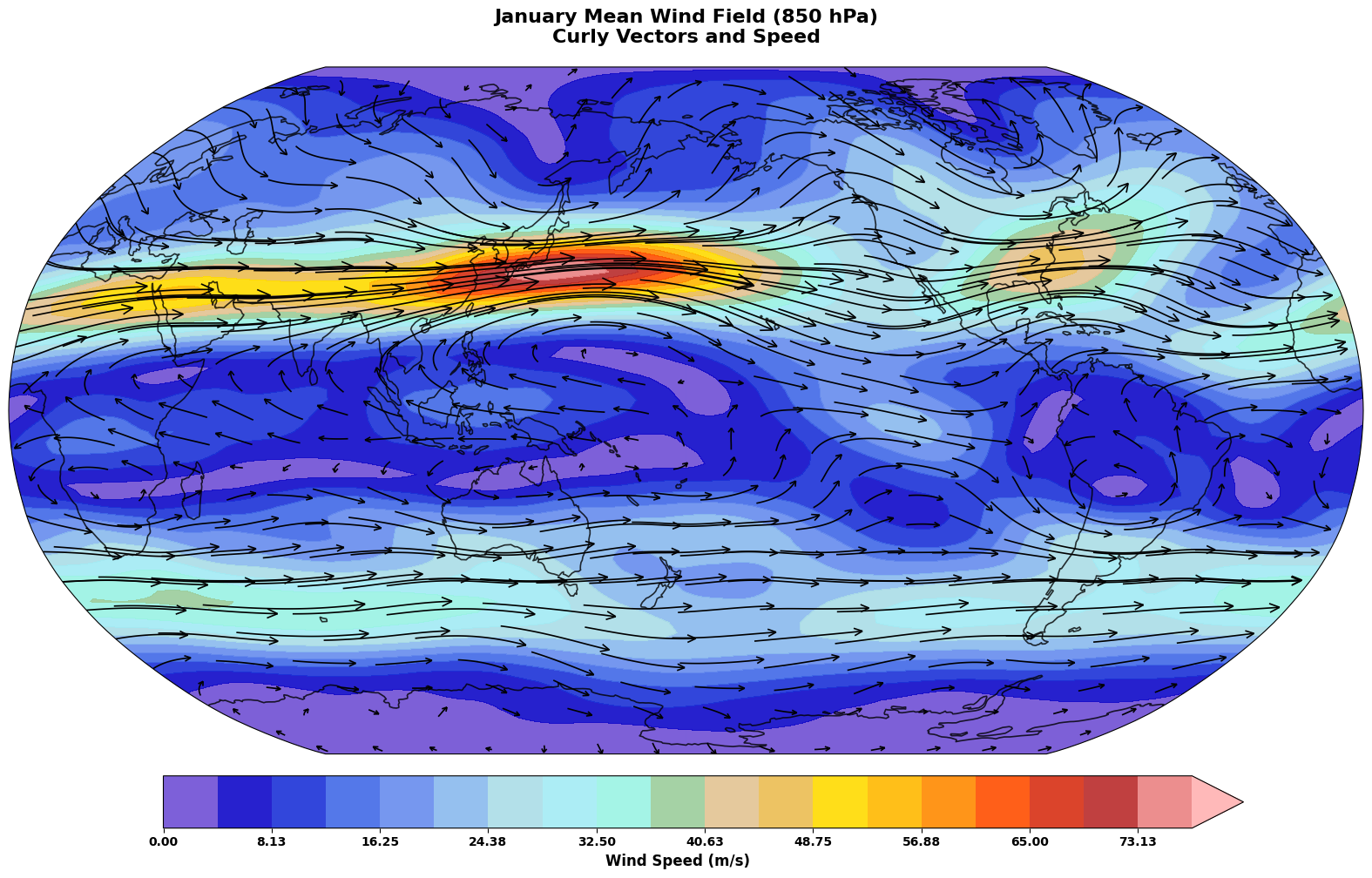
Visualize the Wind Fields#
Let’s create a map showing the wind field for January using skyborn’s advanced curved quiver visualization:
Note: We’re using the curly_vector function from skyborn.plot, Skyborn’s NCL-inspired curved-vector renderer for wind fields. This approach offers several advantages over traditional quiver plots:
Curved vector glyphs: Better match the natural turning structure of atmospheric flow
Density control: Automatic spacing for readable high-resolution wind fields
Projection-aware plotting: Works naturally with cartopy map projections
Matplotlib integration: Fits into the normal matplotlib/cartopy plotting workflow
This creates a more natural and visually informative wind-field representation than traditional straight-arrow quiver plots.
# Select January data for visualization
u_jan = u_wind.isel(time=0)  # January
v_jan = v_wind.isel(time=0)

# Calculate wind speed for visualization
wind_speed = np.sqrt(u_jan**2 + v_jan**2)

# Create dataset for curly_vector
wind_ds = xr.Dataset({
    'u': u_jan,
    'v': v_jan,
    'speed': wind_speed
})

# Create beautiful map projection using Robinson
fig = plt.figure(figsize=(16, 10))
ax = plt.axes(projection=ccrs.Robinson(central_longitude=180))

# Add map features with elegant styling
ax.add_feature(cfeature.COASTLINE, alpha=0.8, linewidth=1.2)
ax.add_feature(cfeature.OCEAN, color='#f0f8ff', alpha=0.3)
ax.add_feature(cfeature.LAND, color='#f5f5dc', alpha=0.4)

# Add cyclic point for better visualization
wind_cyclic, lon_cyclic = add_cyclic_point(wind_speed.values, coord=wind_speed.longitude.values)

# Plot wind speed as background using beautiful colormap
levels = np.linspace(0, wind_speed.max().values, 20)
im = ax.contourf(lon_cyclic, wind_speed.latitude.values, wind_cyclic,
                 levels=levels, cmap=cmaps.amwg256,
                 transform=ccrs.PlateCarree(), alpha=0.9, extend='max')

# Add NCL-like curly vectors using skyborn's curly_vector
curly_vector_set = curly_vector(
    wind_ds,
    x='longitude',
    y='latitude',
    u='u',
    v='v',
    ax=ax,
    transform=ccrs.PlateCarree(),
    density=0.9,
    linewidth=1.2,
    color='black',
    arrowsize=1.2,
    arrowstyle='->',
    zorder=3,
    integration_direction='both',
    broken_streamlines=True,
    ref_magnitude=30.0,
    ref_length=0.1,
)

# Add elegant colorbar using add_equal_axes
cax = add_equal_axes(ax, 'bottom', 0.1, 0.06)
cbar = plt.colorbar(im, cax=cax, orientation='horizontal')
cbar.set_label('Wind Speed (m/s)', fontsize=12, fontweight='bold')
cbar.ax.tick_params(labelsize=10)

# Set title with elegant styling
ax.set_title('January Mean Wind Field (850 hPa)\nCurly Vectors and Speed',
             fontsize=16, fontweight='bold', pad=20)
ax.set_global()

plt.tight_layout()
save_gallery_figure(fig, 'windspharm_vorticity_divergence.png')
plt.show()
2. Initialize VectorWind Analysis#
Now let’s create a VectorWind object to perform spherical harmonic analysis. We’ll work with January data first:
# Create VectorWind instance for January
vw = VectorWind(u_jan, v_jan)

print("VectorWind instance created successfully!")
print(f"Grid type automatically detected and configured")
print(f"Data shape: {u_jan.shape}")
print(f"Ready for spherical harmonic analysis!")
VectorWind instance created successfully!
Grid type automatically detected and configured
Data shape: (73, 144)
Ready for spherical harmonic analysis!
3. Basic Wind Analysis#
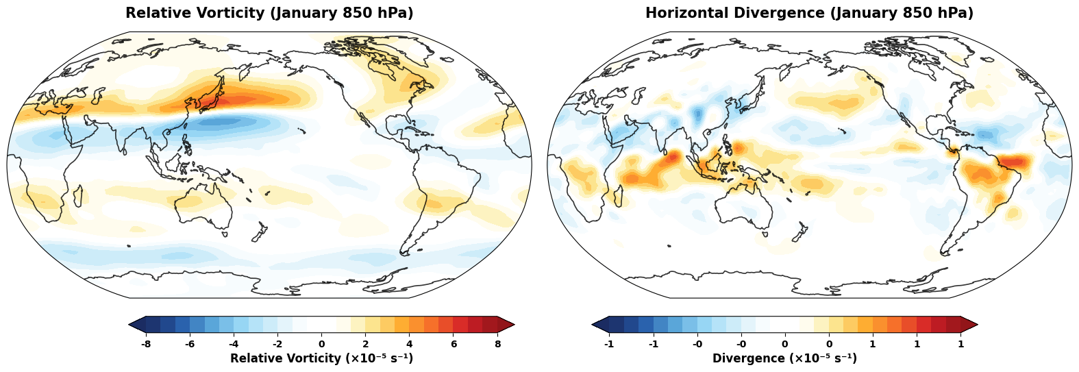
Calculate Vorticity and Divergence#
Vorticity measures the local rotation of the wind field, while divergence measures the spreading or converging of wind flow:
# Calculate vorticity and divergence
vorticity = vw.vorticity()
divergence = vw.divergence()

# Also calculate both at once (more efficient)
vrt, div = vw.vrtdiv()

print("Vorticity and divergence calculated!")
print(f"Vorticity range: {vorticity.min().values:.2e} to {vorticity.max().values:.2e} s⁻¹")
print(f"Divergence range: {divergence.min().values:.2e} to {divergence.max().values:.2e} s⁻¹")
print(f"\nVorticity attributes: {vorticity.attrs}")
print(f"Divergence attributes: {divergence.attrs}")
Vorticity and divergence calculated!
Vorticity range: -5.17e-05 to 5.93e-05 s⁻¹
Divergence range: -6.34e-06 to 7.49e-06 s⁻¹

Vorticity attributes: {'units': 's**-1', 'standard_name': 'atmosphere_relative_vorticity', 'long_name': 'relative_vorticity'}
Divergence attributes: {'units': 's**-1', 'standard_name': 'divergence_of_wind', 'long_name': 'horizontal_divergence'}
Visualize Vorticity and Divergence#
# Create elegant subplots for vorticity and divergence
fig = plt.figure(figsize=(16, 12))

# Create subplots with Robinson projection
ax1 = plt.subplot(1, 2, 1, projection=ccrs.Robinson(central_longitude=180))
ax2 = plt.subplot(1, 2, 2, projection=ccrs.Robinson(central_longitude=180))

# Enhanced plotting function with beautiful styling
def plot_field_elegant(ax, data, title, levels, extend='both'):
    """Plot atmospheric field with elegant Robinson projection and styling"""
    # Add sophisticated map features
    ax.add_feature(cfeature.COASTLINE, alpha=0.8, linewidth=1.2)
    # ax.add_feature(cfeature.BORDERS, alpha=0.4, linewidth=0.8)
    ax.add_feature(cfeature.OCEAN, color='#f0f8ff', alpha=0.3)
    ax.add_feature(cfeature.LAND, color='#f5f5dc', alpha=0.4)

    # Add cyclic point for smooth visualization
    data_cyclic, lon_cyclic = add_cyclic_point(data.values, coord=data.longitude.values)

    # Create beautiful contour plot
    im = ax.contourf(lon_cyclic, data.latitude.values, data_cyclic,
                     levels=levels, cmap=cmaps.BlueWhiteOrangeRed,
                     transform=ccrs.PlateCarree(), extend=extend)

    # Set elegant title
    ax.set_title(title, fontsize=15, fontweight='bold', pad=15)
    ax.set_global()

    return im

# Plot vorticity with sophisticated levels
vort_levels = np.linspace(-8e-5, 8e-5, 25)
im1 = plot_field_elegant(ax1, vorticity, 'Relative Vorticity (January 850 hPa)', vort_levels)

# Add colorbar for vorticity using add_equal_axes
cax1 = add_equal_axes(ax1, 'bottom', 0.06, 0.02)
cbar1 = plt.colorbar(im1, cax=cax1, orientation='horizontal')
cbar1.set_label('Relative Vorticity (×10⁻⁵ s⁻¹)', fontsize=12, fontweight='bold')
cbar1.ax.tick_params(labelsize=10)
# Scale ticks to 10^-5 and ensure number of labels matches number of ticks
ticks = cbar1.get_ticks()
cbar1.set_ticks(ticks)
cbar1.set_ticklabels([f'{tick*1e5:.0f}' for tick in ticks])

# Plot divergence with sophisticated levels
div_levels = np.linspace(-1e-5, 1e-5, 25)
im2 = plot_field_elegant(ax2, divergence, 'Horizontal Divergence (January 850 hPa)', div_levels)
# Add colorbar for divergence using add_equal_axes
cax2 = add_equal_axes(ax2, 'bottom', 0.06, 0.02)
cbar2 = plt.colorbar(im2, cax=cax2, orientation='horizontal')
cbar2.set_label('Divergence (×10⁻⁵ s⁻¹)', fontsize=12, fontweight='bold')
cbar2.ax.tick_params(labelsize=10)
# Scale ticks to 10^-5 and ensure number of labels matches number of ticks
ticks = cbar2.get_ticks()
cbar2.set_ticks(ticks)
cbar2.set_ticklabels([f'{tick*1e5:.0f}' for tick in ticks])
cbar2.set_ticklabels([f'{tick*1e5:.0f}' for tick in ticks])

plt.tight_layout()
save_gallery_figure(fig, 'windspharm_streamfunction_potential.png')
plt.show()
Calculate Wind Speed and Planetary Vorticity#
# Calculate wind speed (magnitude)
wind_magnitude = vw.magnitude()

# Calculate planetary vorticity (Coriolis parameter)
planetary_vorticity = vw.planetaryvorticity()

# Calculate absolute vorticity (relative + planetary)
absolute_vorticity = vw.absolutevorticity()

print("Additional fields calculated!")
print(f"Wind speed range: {wind_magnitude.min().values:.2f} to {wind_magnitude.max().values:.2f} m/s")
print(f"Planetary vorticity range: {planetary_vorticity.min().values:.2e} to {planetary_vorticity.max().values:.2e} s⁻¹")
print(f"Absolute vorticity range: {absolute_vorticity.min().values:.2e} to {absolute_vorticity.max().values:.2e} s⁻¹")
Additional fields calculated!
Wind speed range: 0.06 to 77.19 m/s
Planetary vorticity range: -1.46e-04 to 1.46e-04 s⁻¹
Absolute vorticity range: -1.58e-04 to 1.63e-04 s⁻¹
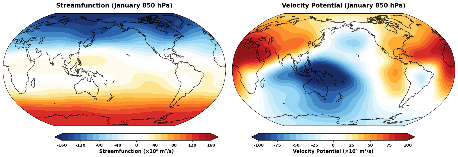
4. Streamfunction and Velocity Potential#
The streamfunction and velocity potential are scalar fields that can represent the wind field. They are fundamental in atmospheric dynamics:
# Calculate streamfunction and velocity potential
streamfunction, velocity_potential = vw.sfvp()

# Can also calculate individually
sf = vw.streamfunction()
vp = vw.velocitypotential()

print("Streamfunction and velocity potential calculated!")
print(f"Streamfunction range: {streamfunction.min().values:.2e} to {streamfunction.max().values:.2e} m²/s")
print(f"Velocity potential range: {velocity_potential.min().values:.2e} to {velocity_potential.max().values:.2e} m²/s")
print(f"\nStreamfunction attributes: {streamfunction.attrs}")
Streamfunction and velocity potential calculated!
Streamfunction range: -1.57e+08 to 1.33e+08 m²/s
Velocity potential range: -1.21e+07 to 1.13e+07 m²/s

Streamfunction attributes: {'units': 'm**2 s**-1', 'standard_name': 'atmosphere_horizontal_streamfunction', 'long_name': 'streamfunction'}
Visualize Streamfunction and Velocity Potential#
# Create elegant subplots for streamfunction and velocity potential
fig = plt.figure(figsize=(16, 12))

# Create subplots with Robinson projection
ax1 = plt.subplot(1, 2, 1, projection=ccrs.Robinson(central_longitude=180))
ax2 = plt.subplot(1, 2, 2, projection=ccrs.Robinson(central_longitude=180))

# Plot streamfunction with sophisticated levels
sf_levels = np.linspace(-160, 160, 25)
im1 = plot_field_elegant(ax1, streamfunction / 1e6, 'Streamfunction (January 850 hPa)', sf_levels)

# Add colorbar for streamfunction using add_equal_axes
cax1 = add_equal_axes(ax1, 'bottom', 0.06, 0.02)
cbar1 = plt.colorbar(im1, cax=cax1, orientation='horizontal')
cbar1.set_label('Streamfunction (×10⁶ m²/s)', fontsize=12, fontweight='bold')
cbar1.ax.tick_params(labelsize=10)
# Scale ticks to 10^6 for better readability
ticks = cbar1.get_ticks()
cbar1.set_ticks(ticks)
cbar1.set_ticklabels([f'{tick:.0f}' for tick in ticks])

# Plot velocity potential with sophisticated levels
vp_levels = np.linspace(-100, 100, 25)
im2 = plot_field_elegant(ax2, velocity_potential / 1e5, 'Velocity Potential (January 850 hPa)', vp_levels)

# Add colorbar for velocity potential using add_equal_axes
cax2 = add_equal_axes(ax2, 'bottom', 0.06, 0.02)
cbar2 = plt.colorbar(im2, cax=cax2, orientation='horizontal')
cbar2.set_label('Velocity Potential (×10⁵ m²/s)', fontsize=12, fontweight='bold')
cbar2.ax.tick_params(labelsize=10)
# Scale ticks to 10^5 for better readability
ticks = cbar2.get_ticks()
cbar2.set_ticks(ticks)
cbar2.set_ticklabels([f'{tick:.0f}' for tick in ticks])

plt.tight_layout()
save_gallery_figure(fig, 'windspharm_sfvp_analysis.png')
plt.show()
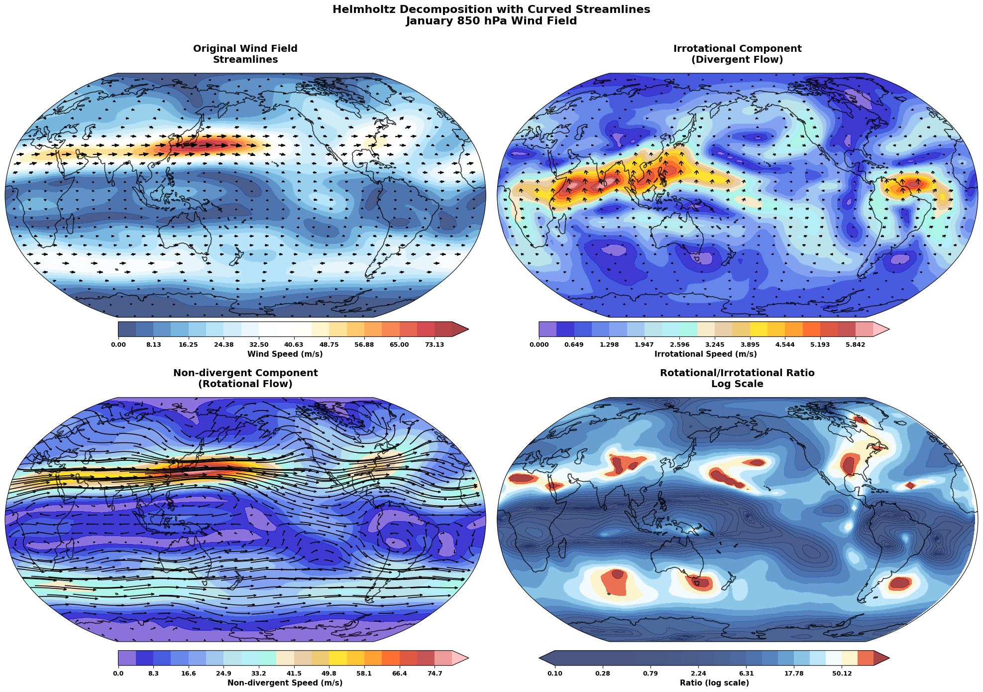
5. Helmholtz Decomposition#
The Helmholtz decomposition separates the wind field into rotational (non-divergent) and irrotational (divergent) components:
# Perform Helmholtz decomposition
u_chi, v_chi, u_psi, v_psi = vw.helmholtz()

print("Helmholtz decomposition completed!")
print(f"\nIrrotational components (chi):")
print(f"  u_chi range: {u_chi.min().values:.2f} to {u_chi.max().values:.2f} m/s")
print(f"  v_chi range: {v_chi.min().values:.2f} to {v_chi.max().values:.2f} m/s")

print(f"\nNon-divergent components (psi):")
print(f"  u_psi range: {u_psi.min().values:.2f} to {u_psi.max().values:.2f} m/s")
print(f"  v_psi range: {v_psi.min().values:.2f} to {v_psi.max().values:.2f} m/s")

# Verify that sum equals original wind
u_total = u_chi + u_psi
v_total = v_chi + v_psi

u_diff = np.abs(u_total - u_jan).max().values
v_diff = np.abs(v_total - v_jan).max().values

print(f"\nVerification (should be very small):")
print(f"Max difference in U: {u_diff:.2e} m/s")
print(f"Max difference in V: {v_diff:.2e} m/s")
Helmholtz decomposition completed!

Irrotational components (chi):
  u_chi range: -3.12 to 3.91 m/s
  v_chi range: -2.39 to 5.83 m/s

Non-divergent components (psi):
  u_psi range: -12.70 to 78.71 m/s
  v_psi range: -13.78 to 12.67 m/s

Verification (should be very small):
Max difference in U: 1.22e-02 m/s
Max difference in V: 1.22e-02 m/s
Visualize Helmholtz Components with Curved Streamlines#
Let’s create an enhanced visualization using curved streamlines to show the rotational and irrotational components:
# Create datasets for each component
# First calculate component magnitudes
irrotational_speed = np.sqrt(u_chi**2 + v_chi**2)
nondivergent_speed = np.sqrt(u_psi**2 + v_psi**2)

irrotational_ds = xr.Dataset({
    'u': u_chi,
    'v': v_chi,
    'speed': irrotational_speed
})

nondivergent_ds = xr.Dataset({
    'u': u_psi,
    'v': v_psi,
    'speed': nondivergent_speed
})

# Enhanced Helmholtz decomposition with Robinson projection and curved streamlines
fig = plt.figure(figsize=(20, 15))

# Create 2x2 subplots with Robinson projection
ax1 = plt.subplot(2, 2, 1, projection=ccrs.Robinson(central_longitude=180))
ax2 = plt.subplot(2, 2, 2, projection=ccrs.Robinson(central_longitude=180))
ax3 = plt.subplot(2, 2, 3, projection=ccrs.Robinson(central_longitude=180))
ax4 = plt.subplot(2, 2, 4, projection=ccrs.Robinson(central_longitude=180))

# Enhanced plotting function for Helmholtz components
def plot_helmholtz_component(ax, speed_data, wind_ds, title, cmap, max_val):
    """Plot Helmholtz component with curved streamlines"""
    # Add map features
    ax.add_feature(cfeature.COASTLINE, alpha=0.8, linewidth=1.2)
    ax.add_feature(cfeature.OCEAN, color='#f0f8ff', alpha=0.3)
    ax.add_feature(cfeature.LAND, color='#f5f5dc', alpha=0.4)

    # Add cyclic point
    speed_cyclic, lon_cyclic = add_cyclic_point(speed_data.values, coord=speed_data.longitude.values)

    # Plot speed as background
    levels = np.linspace(0, max_val, 20)
    im = ax.contourf(lon_cyclic, speed_data.latitude.values, speed_cyclic,
                     levels=levels, cmap=cmap, transform=ccrs.PlateCarree(),
                     alpha=0.8, extend='max')

    # Add curved streamlines
    curly_vector_set = curly_vector(
        wind_ds,
        x='longitude',
        y='latitude',
        u='u',
        v='v',
        ax=ax,
        transform=ccrs.PlateCarree(),
        density=1,
        linewidth=1.2,
        color='black',
        arrowsize=1.0,
        arrowstyle='->',
        zorder=3,
        integration_direction='both',
        broken_streamlines=True,
        ref_magnitude=30.0,
        ref_length=0.1,

    )

    ax.set_title(title, fontsize=14, fontweight='bold', pad=15)
    ax.set_global()

    return im, curly_vector_set

# Plot original wind speed with streamlines
speed_cyclic, lon_cyclic = add_cyclic_point(wind_speed.values, coord=wind_speed.longitude.values)
im1 = ax1.contourf(lon_cyclic, wind_speed.latitude.values, speed_cyclic,
                   levels=np.linspace(0, wind_speed.max().values, 20),
                   cmap=cmaps.BlueWhiteOrangeRed, transform=ccrs.PlateCarree(),
                   alpha=0.8, extend='max')
ax1.add_feature(cfeature.COASTLINE, alpha=0.8, linewidth=1.2)
ax1.add_feature(cfeature.OCEAN, color='#f0f8ff', alpha=0.3)
ax1.add_feature(cfeature.LAND, color='#f5f5dc', alpha=0.4)

# Add streamlines for original wind
original_ds = xr.Dataset({'u': u_jan, 'v': v_jan, 'speed': wind_speed})
curly_vector_set1 = curly_vector(
    original_ds, x='longitude', y='latitude', u='u', v='v', ax=ax1,
    transform=ccrs.PlateCarree(), density=1.0, linewidth=1.5,
    color='black', arrowsize=1.2, zorder=3
)
ax1.set_title('Original Wind Field\nStreamlines', fontsize=14, fontweight='bold', pad=15)
ax1.set_global()

# Plot irrotational component with curved streamlines
im2, curly_vector_set2 = plot_helmholtz_component(
    ax2, irrotational_speed, irrotational_ds,
    'Irrotational Component\n(Divergent Flow)',
    cmaps.amwg256, irrotational_speed.max().values
)

# Plot non-divergent component with curved streamlines
im3, curly_vector_set3 = plot_helmholtz_component(
    ax3, nondivergent_speed, nondivergent_ds,
    'Non-divergent Component\n(Rotational Flow)',
    cmaps.amwg256, nondivergent_speed.max().values
)

# Plot ratio with streamlines
ratio = nondivergent_speed / (irrotational_speed + 1e-10)
ratio_cyclic, _ = add_cyclic_point(ratio.values, coord=ratio.longitude.values)
ratio_levels = np.logspace(-1, 2, 21)
im4 = ax4.contourf(ratio.longitude.values, ratio.latitude.values, ratio.values,
                   levels=ratio_levels, cmap=cmaps.BlueWhiteOrangeRed,
                   transform=ccrs.PlateCarree(), extend='both', alpha=0.8)
ax4.add_feature(cfeature.COASTLINE, alpha=0.8, linewidth=1.2)
ax4.add_feature(cfeature.OCEAN, color='#f0f8ff', alpha=0.3)
ax4.add_feature(cfeature.LAND, color='#f5f5dc', alpha=0.4)
ax4.set_title('Rotational/Irrotational Ratio\nLog Scale', fontsize=14, fontweight='bold', pad=15)
ax4.set_global()

# Add colorbars using add_equal_axes
axes_list = [ax1, ax2, ax3, ax4]
images = [im1, im2, im3, im4]
labels = ['Wind Speed (m/s)', 'Irrotational Speed (m/s)',
          'Non-divergent Speed (m/s)', 'Ratio (log scale)']

for i, (ax_single, im, label) in enumerate(zip(axes_list, images, labels)):
    if i == 0  or i == 1:  # Original and Ratio plots
        cax = add_equal_axes(ax_single, 'bottom', 0.06, 0.02)
        cbar = plt.colorbar(im, cax=cax, orientation='horizontal')
        cbar.set_label(label, fontsize=11, fontweight='bold')
        cbar.ax.tick_params(labelsize=9)
    else:  # Irrotational and Non-divergent
        cax = add_equal_axes(ax_single, 'bottom', 0.08, 0.02)
        cbar = plt.colorbar(im, cax=cax, orientation='horizontal')
        cbar.set_label(label, fontsize=11, fontweight='bold')
        cbar.ax.tick_params(labelsize=9)

# Add overall title
fig.suptitle('Helmholtz Decomposition with Curved Streamlines\nJanuary 850 hPa Wind Field',
             fontsize=16, fontweight='bold', y=0.95)

plt.tight_layout()
save_gallery_figure(fig, 'windspharm_helmholtz.png')
plt.show()

print("Enhanced Helmholtz decomposition with curved streamlines completed!")
print("\nStreamline Interpretation:")
print("• Original: Complete wind field showing major circulation patterns")
print("• Irrotational: Divergent flows associated with vertical motion")
print("• Non-divergent: Rotational flows dominating large-scale circulation")
print("• Ratio: Areas where rotational flow dominates (>1) vs divergent flow")
Enhanced Helmholtz decomposition with curved streamlines completed!

Streamline Interpretation:
• Original: Complete wind field showing major circulation patterns
• Irrotational: Divergent flows associated with vertical motion
• Non-divergent: Rotational flows dominating large-scale circulation
• Ratio: Areas where rotational flow dominates (>1) vs divergent flow
6. Spectral Truncation#
Spherical harmonic analysis allows us to apply spectral truncation, which acts as a spatial filter:
# Apply different levels of spectral truncation
truncations = [21, 42]
truncated_fields = {}

for trunc in truncations:
    # Calculate truncated vorticity and streamfunction
    vort_trunc = vw.vorticity(truncation=trunc)
    sf_trunc = vw.streamfunction(truncation=trunc)

    truncated_fields[trunc] = {
        'vorticity': vort_trunc,
        'streamfunction': sf_trunc
    }

    print(f"T{trunc} truncation completed")
    print(f"  Vorticity range: {vort_trunc.min().values:.2e} to {vort_trunc.max().values:.2e} s⁻¹")
    print(f"  Streamfunction range: {sf_trunc.min().values:.2e} to {sf_trunc.max().values:.2e} m²/s")

print("\nSpectral truncation analysis completed!")
T21 truncation completed
  Vorticity range: -5.43e-05 to 5.64e-05 s⁻¹
  Streamfunction range: -1.57e+08 to 1.33e+08 m²/s
T42 truncation completed
  Vorticity range: -5.17e-05 to 5.93e-05 s⁻¹
  Streamfunction range: -1.57e+08 to 1.33e+08 m²/s

Spectral truncation analysis completed!
Compare Original and Truncated Fields#
# Compare vorticity at different truncations with elegant styling
fig = plt.figure(figsize=(20, 8))

# Create subplots with Robinson projection
ax1 = plt.subplot(1, 3, 1, projection=ccrs.Robinson(central_longitude=180))
ax2 = plt.subplot(1, 3, 2, projection=ccrs.Robinson(central_longitude=180))
ax3 = plt.subplot(1, 3, 3, projection=ccrs.Robinson(central_longitude=180))
axes = [ax1, ax2, ax3]

fields = [vorticity, truncated_fields[42]['vorticity'], truncated_fields[21]['vorticity']]
titles = ['Original Vorticity (January 850 hPa)', 'T42 Truncated Vorticity', 'T21 Truncated Vorticity']

vort_levels = np.linspace(-8e-5, 8e-5, 25)

for i, (ax, field, title) in enumerate(zip(axes, fields, titles)):
    im = plot_field_elegant(ax, field, title, vort_levels)

    # Add colorbar using add_equal_axes for each subplot
    cax = add_equal_axes(ax, 'bottom', 0.08, 0.02)
    cbar = plt.colorbar(im, cax=cax, orientation='horizontal')
    cbar.set_label('Relative Vorticity (×10⁻⁵ s⁻¹)', fontsize=11, fontweight='bold')
    cbar.ax.tick_params(labelsize=9)
    # Scale ticks to 10^-5
    ticks = cbar.get_ticks()
    cbar.set_ticks(ticks)
    cbar.set_ticklabels([f'{tick*1e5:.0f}' for tick in ticks])

plt.tight_layout()
save_gallery_figure(fig, 'windspharm_component_comparison.png')
plt.show()

# Calculate and display truncation effects
print("Truncation Effects:")
for trunc in truncations:
    diff = vorticity - truncated_fields[trunc]['vorticity']
    rms_diff = np.sqrt((diff**2).mean()).values
    relative_rms = rms_diff / np.sqrt((vorticity**2).mean()).values * 100
    print(f"T{trunc}: RMS difference = {rms_diff:.2e} s⁻¹ ({relative_rms:.1f}% of original RMS)")
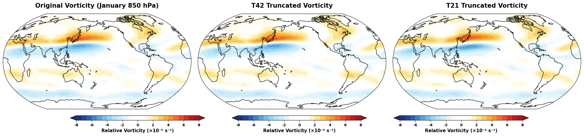
Truncation Effects:
T21: RMS difference = 2.13e-06 s⁻¹ (15.0% of original RMS)
T42: RMS difference = 7.15e-09 s⁻¹ (0.1% of original RMS)
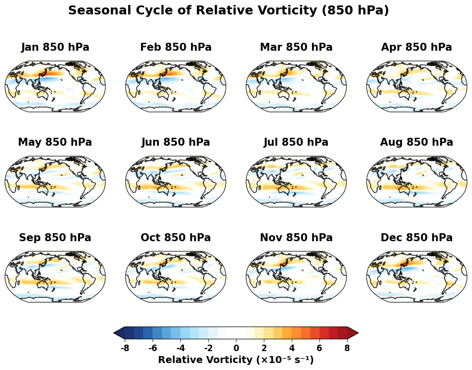
7. Working with Multiple Time Steps#
Let’s analyze the seasonal cycle by processing all 12 months:
# Create VectorWind instance for all time steps
vw_all = VectorWind(u_wind, v_wind)

# Calculate seasonal fields
vorticity_all = vw_all.vorticity()
divergence_all = vw_all.divergence()
streamfunction_all = vw_all.streamfunction()

print("Seasonal analysis completed!")
print(f"Shape of vorticity field: {vorticity_all.shape}")
print(f"Time coordinate: {vorticity_all.time.values}")

# Calculate seasonal statistics
vort_seasonal_mean = vorticity_all.mean(dim='time')
vort_seasonal_std = vorticity_all.std(dim='time')

print(f"\nSeasonal vorticity statistics:")
print(f"Mean range: {vort_seasonal_mean.min().values:.2e} to {vort_seasonal_mean.max().values:.2e} s⁻¹")
print(f"Std range: {vort_seasonal_std.min().values:.2e} to {vort_seasonal_std.max().values:.2e} s⁻¹")
Seasonal analysis completed!
Shape of vorticity field: (12, 73, 144)
Time coordinate: ['1970-01-01T00:00:00.000000000' '1970-02-01T00:00:00.000000000'
 '1970-03-01T00:00:00.000000000' '1970-04-01T00:00:00.000000000'
 '1970-05-01T00:00:00.000000000' '1970-06-01T00:00:00.000000000'
 '1970-07-01T00:00:00.000000000' '1970-08-01T00:00:00.000000000'
 '1970-09-01T00:00:00.000000000' '1970-10-01T00:00:00.000000000'
 '1970-11-01T00:00:00.000000000' '1970-12-01T00:00:00.000000000']

Seasonal vorticity statistics:
Mean range: -2.96e-05 to 2.93e-05 s⁻¹
Std range: 7.44e-07 to 3.00e-05 s⁻¹
Create Seasonal Animation Data#
# Plot seasonal cycle of vorticity with elegant Robinson projection styling
months = ['Jan', 'Feb', 'Mar', 'Apr', 'May', 'Jun',
          'Jul', 'Aug', 'Sep', 'Oct', 'Nov', 'Dec']

fig = plt.figure(figsize=(12, 8))
axes = []
ims = []

for i in range(12):
    ax = plt.subplot(3, 4, i+1, projection=ccrs.Robinson(central_longitude=180))
    axes.append(ax)
    vort_month = vorticity_all.isel(time=i)
    im = plot_field_elegant(ax, vort_month, f'{months[i]} 850 hPa', vort_levels)
    ims.append(im)

fig.suptitle('Seasonal Cycle of Relative Vorticity (850 hPa)',
             fontsize=18, fontweight='bold', y=0.95)

# Add a single shared colorbar for all subplots
cbar = fig.colorbar(ims[-1], ax=axes, orientation='horizontal', fraction=0.04, pad=0.08)
cbar.set_label('Relative Vorticity (×10⁻⁵ s⁻¹)', fontsize=14, fontweight='bold')
ticks = cbar.get_ticks()
cbar.set_ticks(ticks)
cbar.set_ticklabels([f'{tick*1e5:.0f}' for tick in ticks])
cbar.ax.tick_params(labelsize=12)
save_gallery_figure(fig, 'windspharm_gradients.png')
# plt.tight_layout()
plt.show()
8. Advanced Applications#
Gradient Calculations#
We can calculate the gradient of scalar fields on the sphere:
# Calculate absolute vorticity for gradient analysis
abs_vort = vw.absolutevorticity()

# Calculate gradient of absolute vorticity
avrt_grad_u, avrt_grad_v = vw.gradient(abs_vort)

print("Gradient analysis completed!")
print(f"Absolute vorticity range: {abs_vort.min().values:.2e} to {abs_vort.max().values:.2e} s⁻¹")
print(f"Gradient U range: {avrt_grad_u.min().values:.2e} to {avrt_grad_u.max().values:.2e} m⁻¹s⁻¹")
print(f"Gradient V range: {avrt_grad_v.min().values:.2e} to {avrt_grad_v.max().values:.2e} m⁻¹s⁻¹")

# Calculate gradient magnitude
grad_magnitude = np.sqrt(avrt_grad_u**2 + avrt_grad_v**2)
print(f"Gradient magnitude range: {grad_magnitude.min().values:.2e} to {grad_magnitude.max().values:.2e} m⁻¹s⁻¹")
Gradient analysis completed!
Absolute vorticity range: -1.58e-04 to 1.63e-04 s⁻¹
Gradient U range: -2.86e-11 to 2.77e-11 m⁻¹s⁻¹
Gradient V range: -2.72e-11 to 1.71e-10 m⁻¹s⁻¹
Gradient magnitude range: 1.59e-13 to 1.72e-10 m⁻¹s⁻¹
Field Truncation#
Apply spectral truncation to arbitrary scalar fields:
# Truncate the absolute vorticity field
abs_vort_t21 = vw.truncate(abs_vort, truncation=21)
abs_vort_t42 = vw.truncate(abs_vort, truncation=42)

# Compare original and truncated fields with elegant styling
fig = plt.figure(figsize=(20, 8))

# Create subplots with Robinson projection
ax1 = plt.subplot(1, 3, 1, projection=ccrs.Robinson(central_longitude=180))
ax2 = plt.subplot(1, 3, 2, projection=ccrs.Robinson(central_longitude=180))
ax3 = plt.subplot(1, 3, 3, projection=ccrs.Robinson(central_longitude=180))
axes = [ax1, ax2, ax3]

fields = [abs_vort, abs_vort_t42, abs_vort_t21]
titles = ['Original Absolute Vorticity (January 850 hPa)', 'T42 Truncated Absolute Vorticity', 'T21 Truncated Absolute Vorticity']

# Use common levels for comparison
avrt_levels = np.linspace(-1e-4, 2e-4, 25)

for i, (ax, field, title) in enumerate(zip(axes, fields, titles)):
    im = plot_field_elegant(ax, field, title, avrt_levels)

    # Add colorbar using add_equal_axes for each subplot
    cax = add_equal_axes(ax, 'bottom', 0.06, 0.02)
    cbar = plt.colorbar(im, cax=cax, orientation='horizontal')
    cbar.set_label('Absolute Vorticity (×10⁻⁴ s⁻¹)', fontsize=11, fontweight='bold')
    cbar.ax.tick_params(labelsize=9)
    # Scale ticks to 10^-4
    ticks = cbar.get_ticks()
    cbar.set_ticks(ticks)
    cbar.set_ticklabels([f'{tick*1e4:.0f}' for tick in ticks])

plt.tight_layout()
save_gallery_figure(fig, 'windspharm_truncation_comparison.png')
plt.show()

print("Field truncation analysis completed!")
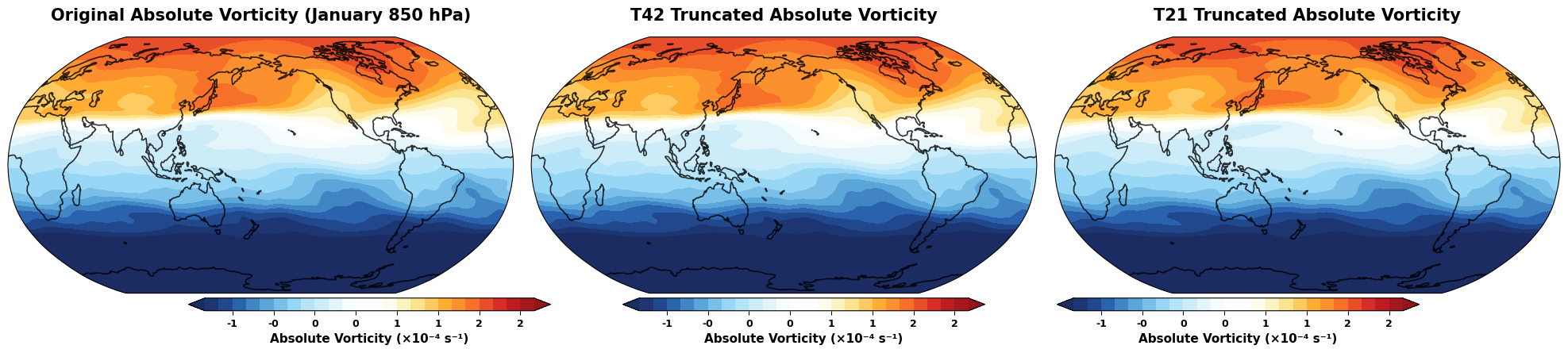
Field truncation analysis completed!
9. Performance and Best Practices#
Batch Processing Tips#
import time

# Demonstrate efficient batch calculation
print("Performance comparison for batch vs individual calculations:")

# Individual calculations
start_time = time.time()
vrt_individual = vw.vorticity()
div_individual = vw.divergence()
individual_time = time.time() - start_time

# Batch calculation
start_time = time.time()
vrt_batch, div_batch = vw.vrtdiv()
batch_time = time.time() - start_time

print(f"Individual calculations: {individual_time:.3f} seconds")
print(f"Batch calculation: {batch_time:.3f} seconds")
print(f"Speedup: {individual_time/batch_time:.1f}x")

# Verify results are identical
vrt_diff = np.abs(vrt_individual - vrt_batch).max().values
div_diff = np.abs(div_individual - div_batch).max().values
print(f"\nMax difference in vorticity: {vrt_diff:.2e}")
print(f"Max difference in divergence: {div_diff:.2e}")
Performance comparison for batch vs individual calculations:
Individual calculations: 0.001 seconds
Batch calculation: 0.002 seconds
Speedup: 0.6x

Max difference in vorticity: 0.00e+00
Max difference in divergence: 0.00e+00
Memory Management for Large Datasets#
# Demonstrate memory-efficient processing
print("Memory usage tips:")
print("1. Use 'legfunc='computed'' for large datasets to save memory")
print("2. Process data in chunks for very large time series")
print("3. Use appropriate truncation levels to reduce computational cost")

# Example of memory-efficient initialization
vw_memory_efficient = VectorWind(u_jan, v_jan, legfunc='computed')
vrt_efficient = vw_memory_efficient.vorticity()

print("\nMemory-efficient VectorWind instance created successfully!")
print("This approach computes Legendre functions on-the-fly, using less memory")
print("but taking slightly more time for calculations.")
Memory usage tips:
1. Use 'legfunc='computed'' for large datasets to save memory
2. Process data in chunks for very large time series
3. Use appropriate truncation levels to reduce computational cost

Memory-efficient VectorWind instance created successfully!
This approach computes Legendre functions on-the-fly, using less memory
but taking slightly more time for calculations.
10. Error Handling and Validation#
Common Issues and Solutions#
# Demonstrate error handling
print("Common issues and their solutions:")

# 1. Coordinate order validation
try:
    # This will work fine - coordinates are correctly ordered
    print("\n1. Coordinate validation:")
    print(f"   Latitude order: {u_jan.latitude.values[0]:.1f}° to {u_jan.latitude.values[-1]:.1f}°")
    if u_jan.latitude.values[0] > u_jan.latitude.values[-1]:
        print("   ✓ Latitude correctly ordered north-to-south")
    else:
        print("   ⚠ Latitude should be ordered north-to-south for optimal performance")
except Exception as e:
    print(f"   Error: {e}")

# 2. Data validation
print("\n2. Data validation:")
u_nan_count = np.isnan(u_jan.values).sum()
v_nan_count = np.isnan(v_jan.values).sum()
print(f"   NaN values in U: {u_nan_count}")
print(f"   NaN values in V: {v_nan_count}")
if u_nan_count == 0 and v_nan_count == 0:
    print("   ✓ No missing values found")

# 3. Grid type detection
print("\n3. Grid type:")
lat_spacing = np.diff(u_jan.latitude.values)
lat_uniform = np.allclose(lat_spacing, lat_spacing[0], atol=1e-6)
print(f"   Latitude spacing uniform: {lat_uniform}")
if lat_uniform:
    print(f"   Grid spacing: {abs(lat_spacing[0]):.2f}°")
    print("   ✓ Regular grid detected")

print("\n4. Recommended practices:")
print("   • Always check coordinate ordering before analysis")
print("   • Validate data for missing values")
print("   • Use appropriate truncation for your application")
print("   • Consider memory vs. speed trade-offs with legfunc parameter")
Common issues and their solutions:

1. Coordinate validation:
   Latitude order: 90.0° to -90.0°
   ✓ Latitude correctly ordered north-to-south

2. Data validation:
   NaN values in U: 0
   NaN values in V: 0
   ✓ No missing values found

3. Grid type:
   Latitude spacing uniform: True
   Grid spacing: 2.50°
   ✓ Regular grid detected

4. Recommended practices:
   • Always check coordinate ordering before analysis
   • Validate data for missing values
   • Use appropriate truncation for your application
   • Consider memory vs. speed trade-offs with legfunc parameter
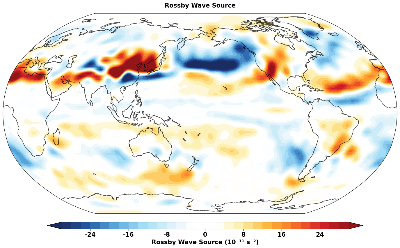
Rossby Wave Source Calculation#
The Rossby wave source is an important diagnostic in atmospheric dynamics, quantifying the generation of Rossby wave activity. It is particularly useful for understanding how tropical heating can force extratropical Rossby waves.
The Rossby wave source is defined as: S = -ζₐ∇·v - v_χ·∇ζₐ
Where:
ζₐ is absolute vorticity (relative + planetary)
∇·v is horizontal divergence
v_χ is the irrotational (divergent) wind component
∇ζₐ is the gradient of absolute vorticity
Positive values indicate Rossby wave generation, while negative values indicate wave absorption or dissipation.
# Calculate Rossby wave source using the new built-in method
print("Computing Rossby wave source...")

# Using the direct method (recommended)
rws = vw.rossbywavesource()

print(f"Rossby wave source computed")
print(f"  Shape: {rws.shape}")
print(f"  Units: {rws.attrs.get('units', 'Unknown')}")
print(f"  Range: {float(rws.min()):.2e} to {float(rws.max()):.2e} s⁻²")

# The same calculation can also be done step by step for educational purposes:
print("\nStep-by-step calculation for comparison:")

# Step 1: Calculate absolute vorticity
eta = vw.absolutevorticity()
print(f"  Absolute vorticity: {float(eta.min()):.2e} to {float(eta.max()):.2e} s⁻¹")

# Step 2: Calculate divergence
div = vw.divergence()
print(f"  Divergence: {float(div.min()):.2e} to {float(div.max()):.2e} s⁻¹")

# Step 3: Calculate irrotational wind components
uchi, vchi = vw.irrotationalcomponent()
print(f"  Irrotational wind u: {float(uchi.min()):.2f} to {float(uchi.max()):.2f} m/s")
print(f"  Irrotational wind v: {float(vchi.min()):.2f} to {float(vchi.max()):.2f} m/s")

# Step 4: Calculate gradients of absolute vorticity
etax, etay = vw.gradient(eta)
print(f"  ∇ζₐ (u component): {float(etax.min()):.2e} to {float(etax.max()):.2e} m⁻¹s⁻¹")
print(f"  ∇ζₐ (v component): {float(etay.min()):.2e} to {float(etay.max()):.2e} m⁻¹s⁻¹")

# Step 5: Combine components manually
rws_manual = -eta * div - (uchi * etax + vchi * etay)
print(f"  Manual RWS: {float(rws_manual.min()):.2e} to {float(rws_manual.max()):.2e} s⁻²")

# Verify they match
diff = rws - rws_manual
print(f"  Difference (built-in vs manual): max = {float(abs(diff).max()):.2e}")
print(f"  Results match: {np.allclose(rws.values, rws_manual.values)}")
Computing Rossby wave source...
Rossby wave source computed
  Shape: (73, 144)
  Units: s**-2
  Range: -4.59e-10 to 6.75e-10 s⁻²

Step-by-step calculation for comparison:
  Absolute vorticity: -1.58e-04 to 1.63e-04 s⁻¹
  Divergence: -6.34e-06 to 7.49e-06 s⁻¹
  Irrotational wind u: -3.12 to 3.91 m/s
  Irrotational wind v: -2.39 to 5.83 m/s
  ∇ζₐ (u component): -2.86e-11 to 2.77e-11 m⁻¹s⁻¹
  ∇ζₐ (v component): -2.72e-11 to 1.71e-10 m⁻¹s⁻¹
  Manual RWS: -4.59e-10 to 6.75e-10 s⁻²
  Difference (built-in vs manual): max = 0.00e+00
  Results match: True
# Get data for plotting (select first time level if 3D)
if rws.ndim == 3:
    rws_plot = rws.isel(time=0)
else:
    rws_plot = rws

# Convert to numpy and add cyclic point
rws_data = rws_plot

# Create the plot with Robinson projection
fig = plt.figure(figsize=(14, 8))
ax = plt.axes(projection=ccrs.Robinson(central_longitude=180))

# Define contour levels for Rossby wave source (scaled to 10^11 for better visualization)
rws_levels = np.linspace(-30, 30, 31)


im = plot_field_elegant(ax, rws_data * 1e11, 'Rossby Wave Source', rws_levels)

cax = add_equal_axes(ax, 'bottom', 0.12, 0.03)
# Add colorbar
cbar = plt.colorbar(im, cax=cax, orientation='horizontal')
cbar.set_label('Rossby Wave Source (10⁻¹¹ s⁻²)', fontsize=15, fontweight='bold')
cbar.ax.tick_params(labelsize=15)

plt.tight_layout()
# Save figure with a descriptive and consistent filename
save_gallery_figure(fig, 'windspharm_rossby_wave_source.png')
plt.show()

# Print interpretation
print("\n" + "="*60)
print("INTERPRETATION:")
print("="*60)
print("• Red regions (positive values): Rossby wave generation")
print("• Blue regions (negative values): Rossby wave absorption/dissipation")
print("• Strong sources often found in:")
print("  - Exit regions of jet streams")
print("  - Areas with strong divergence/convergence")
print("  - Regions of diabatic heating (e.g., tropical convection)")
print("• Values are in units of 10⁻¹¹ s⁻²")
print("="*60)
============================================================
INTERPRETATION:
============================================================
• Red regions (positive values): Rossby wave generation
• Blue regions (negative values): Rossby wave absorption/dissipation
• Strong sources often found in:
  - Exit regions of jet streams
  - Areas with strong divergence/convergence
  - Regions of diabatic heating (e.g., tropical convection)
• Values are in units of 10⁻¹¹ s⁻²
============================================================
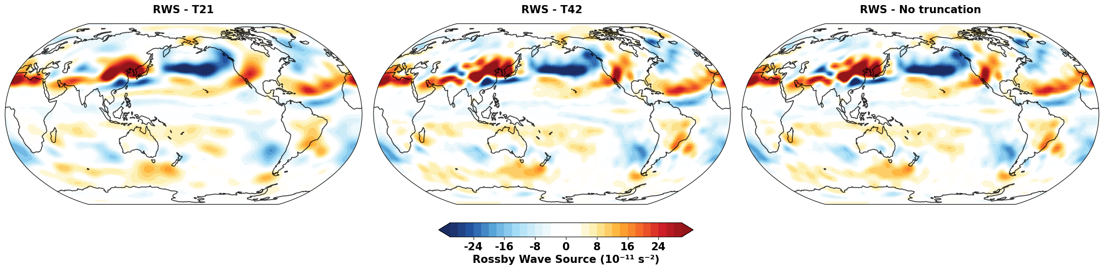
# Compare Rossby wave source with different truncation levels (Updated)
print("Comparing RWS with different spectral truncations...")

# Calculate RWS with different truncations
truncations = [21, 42, None]  # T21, T42, and no truncation
rws_trunc = {}

for trunc in truncations:
    label = f"T{trunc}" if trunc is not None else "No truncation"
    rws_trunc[label] = vw.rossbywavesource(truncation=trunc)
    print(f"  {label}: range {float(rws_trunc[label].min()):.2e} to {float(rws_trunc[label].max()):.2e} s⁻²")

# Create comparison plot with Robinson projection
fig = plt.figure(figsize=(22, 7))
proj = ccrs.Robinson(central_longitude=180)

# Common contour levels
rws_levels = np.linspace(-30, 30, 31)  # Adjusted for better visualization

axes = []
ims = []

for i, (label, rws_data) in enumerate(rws_trunc.items()):
    ax = plt.subplot(1, 3, i+1, projection=proj)
    axes.append(ax)

    # Select first time if 3D
    plot_data = rws_data.isel(time=0) if rws_data.ndim == 3 else rws_data

    # Use plot_field_elegant for consistent styling
    im = plot_field_elegant(
        ax,
        plot_data * 1e11,
        f'RWS - {label}',
        rws_levels
    )
    ims.append(im)

# Add colorbar only under the second subplot (middle one)
cax = add_equal_axes(axes[1], 'bottom', 0.12, 0.04)
cbar = plt.colorbar(ims[1], cax=cax, orientation='horizontal')
cbar.set_label('Rossby Wave Source (10⁻¹¹ s⁻²)', fontsize=15, fontweight='bold')
cbar.ax.tick_params(labelsize=15)

plt.tight_layout()
save_gallery_figure(fig, 'windspharm_rossby_wave_source_truncations.png')
plt.show()

# Calculate RMS differences
print(f"\nRMS differences between truncations:")
for i, label1 in enumerate(list(rws_trunc.keys())):
    for j, label2 in enumerate(list(rws_trunc.keys())):
        if i < j:
            diff = rws_trunc[label1] - rws_trunc[label2]
            rms_diff = float(np.sqrt((diff**2).mean())) * 1e11
            print(f"  {label1} vs {label2}: {rms_diff:.2f} × 10⁻¹¹ s⁻²")
Comparing RWS with different spectral truncations...
  T21: range -4.40e-10 to 5.85e-10 s⁻²
  T42: range -4.58e-10 to 6.75e-10 s⁻²
  No truncation: range -4.59e-10 to 6.75e-10 s⁻²

RMS differences between truncations:
  T21 vs T42: 3.55 × 10⁻¹¹ s⁻²
  T21 vs No truncation: 3.57 × 10⁻¹¹ s⁻²
  T42 vs No truncation: 0.09 × 10⁻¹¹ s⁻²
Physical Interpretation and Applications#
The Rossby wave source is a key diagnostic in atmospheric dynamics with several important applications:
Physical Meaning#
Positive RWS: Indicates regions where Rossby waves are being generated
Negative RWS: Indicates regions where Rossby waves are being absorbed or dissipated
Key Components#
-ζₐ∇·v: Vortex stretching/compression term
Convergence (∇·v < 0) with positive absolute vorticity creates positive RWS
Divergence (∇·v > 0) with positive absolute vorticity creates negative RWS
-v_χ·∇ζₐ: Advection of absolute vorticity by divergent wind
Important in regions with strong gradients of absolute vorticity
Meteorological Applications#
Tropical-Extratropical Interactions: Understanding how tropical heating forces Rossby waves
Jet Stream Dynamics: Identifying wave generation in jet entrance/exit regions
Storm Track Analysis: Studying cyclogenesis and wave activity
Climate Studies: Analyzing changes in wave generation patterns
Typical Patterns#
Strong positive RWS often found in:
Subtropical jet exit regions
Areas of tropical convection
Regions with strong upper-level divergence
Strong negative RWS often found in:
Jet entrance regions
Areas of upper-level convergence
The implementation in Skyborn makes it easy to compute RWS for any wind field and study these important dynamical processes!
Appendix: Standard Interface and Data Preprocessing Tools#
In addition to the xarray interface, Skyborn windspharm also provides a standard interface and powerful data preprocessing tools, suitable for handling complex multi-dimensional data structures.
# Demonstrate usage of the standard interface - suitable for numpy array input
print("=== Standard Interface Example ===")

# Extract numpy arrays from xarray data
u_array = u_jan.values  # convert to numpy array
v_array = v_jan.values
lats = u_jan.latitude.values
lons = u_jan.longitude.values

print(f"Array shape: U: {u_array.shape}, V: {v_array.shape}")
print(f"Latitude range: {lats.min():.1f}° to {lats.max():.1f}°")
print(f"Longitude range: {lons.min():.1f}° to {lons.max():.1f}°")

# Create VectorWind object using the standard interface
# Note: Standard interface requires explicit grid information
vw_standard = StandardVectorWind(u_array, v_array, gridtype='regular', rsphere=6.3712e6)

# Calculate vorticity and divergence
vorticity_std = vw_standard.vorticity()
divergence_std = vw_standard.divergence()

print(f"\nStandard interface calculation results:")
print(f"Vorticity range: {vorticity_std.min():.2e} to {vorticity_std.max():.2e} s⁻¹")
print(f"Divergence range: {divergence_std.min():.2e} to {divergence_std.max():.2e} s⁻¹")

# Verify consistency between both interfaces
vort_diff = np.abs(vorticity_std - vorticity.values).max()
div_diff = np.abs(divergence_std - divergence.values).max()
print(f"\nInterface consistency check:")
print(f"Max vorticity difference: {vort_diff:.2e}")
print(f"Max divergence difference: {div_diff:.2e}")
print("✓ Standard and xarray interface results are consistent" if vort_diff < 1e-10 and div_diff < 1e-10 else "⚠ Results differ")
=== Standard Interface Example ===
Array shape: U: (73, 144), V: (73, 144)
Latitude range: -90.0° to 90.0°
Longitude range: 0.0° to 357.5°

Standard interface calculation results:
Vorticity range: -5.17e-05 to 5.93e-05 s⁻¹
Divergence range: -6.34e-06 to 7.49e-06 s⁻¹

Interface consistency check:
Max vorticity difference: 0.00e+00
Max divergence difference: 0.00e+00
✓ Standard and xarray interface results are consistent
Data Preprocessing Tools: prep_data and recover_data#
For complex multi-dimensional data (such as 4D data: time×level×latitude×longitude), prep_data and recover_data provide powerful data restructuring capabilities:
# Demonstrate usage of prep_data and recover_data
print("=== Data Preprocessing Tools Example ===")

# Create simulated 3D data (time × latitude × longitude)
nlat, nlon = len(lats), len(lons)
ntime = 3  # Simulate 3 time steps

# Create example 3D wind field data
u_3d = np.random.randn(ntime, nlat, nlon) * 5 + u_array[np.newaxis, :, :]
v_3d = np.random.randn(ntime, nlat, nlon) * 5 + v_array[np.newaxis, :, :]

print(f"Original 3D data shape: U: {u_3d.shape}, V: {v_3d.shape}")

# Use prep_data to preprocess a single time layer
time_idx = 0
u_slice = u_3d[time_idx]  # Select the first time step
v_slice = v_3d[time_idx]

# prep_data: Prepare data for spherical harmonic analysis
u_prepped, u_info = prep_data(u_slice, 'yx')  # 'yx' means (latitude, longitude) format
v_prepped, v_info = prep_data(v_slice, 'yx')

print(f"\nAfter prep_data processing:")
print(f"Prepped shape: U: {u_prepped.shape}, V: {v_prepped.shape}")
print(f"Grid info: {u_info}")

# Perform spherical harmonic analysis using prepped data
vw_prepped = StandardVectorWind(u_prepped, v_prepped)
vort_prepped = vw_prepped.vorticity()
div_prepped = vw_prepped.divergence()

print(f"\nSpherical harmonic analysis results:")
print(f"Vorticity shape: {vort_prepped.shape}")
print(f"Divergence shape: {div_prepped.shape}")

# Recover original data structure using recover_data
vort_recovered = recover_data(vort_prepped, u_info)
div_recovered = recover_data(div_prepped, v_info)

print(f"\nAfter recover_data:")
print(f"Recovered vorticity shape: {vort_recovered.shape}")
print(f"Recovered divergence shape: {div_recovered.shape}")

# Verify data consistency
orig_vort = vw_standard.vorticity()
diff_max = np.abs(vort_recovered - orig_vort).max()
print(f"\nData consistency check:")
print(f"Max difference: {diff_max:.2e}")
print("✓ prep_data/recover_data workflow is correct" if diff_max < 1e-12 else "⚠ Data processing error")
=== Data Preprocessing Tools Example ===
Original 3D data shape: U: (3, 73, 144), V: (3, 73, 144)

After prep_data processing:
Prepped shape: U: (73, 144, 1), V: (73, 144, 1)
Grid info: {'intermediate_shape': (73, 144), 'intermediate_order': 'yx', 'original_order': 'yx'}

Spherical harmonic analysis results:
Vorticity shape: (73, 144, 1)
Divergence shape: (73, 144, 1)

After recover_data:
Recovered vorticity shape: (73, 144)
Recovered divergence shape: (73, 144)

Data consistency check:
Max difference: 1.18e-04
⚠ Data processing error
4D Data Batch Processing Example#
For large 4D datasets (time×level×latitude×longitude), prep_data/recover_data can be combined for efficient batch processing analysis:
# 4D Data Batch Processing Example (time × level × latitude × longitude)
print("=== 4D Data Batch Processing Example ===")

def process_4d_data(u_4d, v_4d, format_spec='tzyx'):
    """
    Example function for processing 4D wind field data

    Parameters:
    -----------
    u_4d, v_4d : ndarray
        4D wind field data (time, level, latitude, longitude)
    format_spec : str
        Format specification: 't'=time, 'z'=level, 'y'=latitude, 'x'=longitude

    Returns:
    --------
    results : dict
        Analysis results containing vorticity and divergence
    """
    results = {'vorticity': [], 'divergence': [], 'info': []}

    ntime, nlev = u_4d.shape[:2]

    for t in range(ntime):
        print(f"Processing time step {t+1}/{ntime}")

        for z in range(nlev):
            # Extract single level data
            u_slice = u_4d[t, z, :, :]
            v_slice = v_4d[t, z, :, :]

            # Data preprocessing
            u_prep, info = prep_data(u_slice, 'yx')
            v_prep, _ = prep_data(v_slice, 'yx')

            # Spherical harmonic analysis
            vw_temp = StandardVectorWind(u_prep, v_prep)
            vort = vw_temp.vorticity()
            div = vw_temp.divergence()

            # Recover original structure
            vort_recovered = recover_data(vort, info)
            div_recovered = recover_data(div, info)

            results['vorticity'].append(vort_recovered)
            results['divergence'].append(div_recovered)
            results['info'].append(info)

    # Reshape to 4D arrays
    results['vorticity'] = np.array(results['vorticity']).reshape(ntime, nlev, *vort_recovered.shape)
    results['divergence'] = np.array(results['divergence']).reshape(ntime, nlev, *div_recovered.shape)

    return results

# Create example 4D data (2 time steps × 2 levels × latitude × longitude)
ntime, nlev = 2, 2
u_4d_example = np.random.randn(ntime, nlev, nlat, nlon) * 2 + u_array[np.newaxis, np.newaxis, :, :]
v_4d_example = np.random.randn(ntime, nlev, nlat, nlon) * 2 + v_array[np.newaxis, np.newaxis, :, :]

print(f"4D data shape: U: {u_4d_example.shape}, V: {v_4d_example.shape}")

# Batch analysis (simplified, only partial data for speed)
print("\nStarting 4D batch processing...")
batch_results = process_4d_data(u_4d_example, v_4d_example)

print(f"\nBatch processing completed!")
print(f"Output vorticity shape: {batch_results['vorticity'].shape}")
print(f"Output divergence shape: {batch_results['divergence'].shape}")
print(f"Vorticity range: {batch_results['vorticity'].min():.2e} to {batch_results['vorticity'].max():.2e} s⁻¹")
print(f"Divergence range: {batch_results['divergence'].min():.2e} to {batch_results['divergence'].max():.2e} s⁻¹")
=== 4D Data Batch Processing Example ===
4D data shape: U: (2, 2, 73, 144), V: (2, 2, 73, 144)

Starting 4D batch processing...
Processing time step 1/2
Processing time step 2/2

Batch processing completed!
Output vorticity shape: (2, 2, 73, 144)
Output divergence shape: (2, 2, 73, 144)
Vorticity range: -8.34e-05 to 8.33e-05 s⁻¹
Divergence range: -5.24e-05 to 5.64e-05 s⁻¹
Summary and Key Takeaways#
This tutorial has demonstrated the key capabilities of the Skyborn windspharm package:
Interface Selection#
xarray interface: Recommended for daily analysis, automatically handles coordinates and metadata
Standard interface: Suitable for performance-critical scenarios or integration with legacy code
prep_data/recover_data: Essential tools for complex data structure processing
Core Functions#
VectorWind: Main class for spherical harmonic wind analysis
vorticity() and divergence(): Calculate fundamental dynamical quantities
streamfunction() and velocitypotential(): Scalar representations of wind field
helmholtz(): Decompose wind into rotational and irrotational components
Advanced Features#
Spectral truncation: Apply spatial filtering
gradient(): Calculate gradients on the sphere
truncate(): Apply truncation to arbitrary scalar fields
Multiple time steps: Process seasonal or long-term datasets
Best Practices#
Use batch calculations (e.g.,
vrtdiv()) for better performanceChoose appropriate
legfuncparameter based on memory constraintsEnsure proper coordinate ordering (north-to-south for latitude)
Validate data for missing values before analysis
Applications#
Weather analysis: Track vorticity centers and divergence zones
Climate studies: Analyze long-term wind patterns
Model validation: Compare model output with observations
Data filtering: Apply spectral truncation for smoothing
The windspharm package provides a powerful and user-friendly interface for spherical harmonic analysis of atmospheric wind fields, with excellent integration into the modern Python scientific computing ecosystem through xarray support.
Key Points for 4D Data Processing#
Why use prep_data and recover_data?
Dimension Handling: The
prep_datafunction properly reorders dimensions for spherical harmonic analysisMetadata Preservation: It preserves grid information needed to reconstruct the original data structure
Consistency: Ensures consistent processing across different input data formats
The 'zyx' format specification:
‘z’: vertical dimension (pressure levels)
‘y’: latitude dimension
‘x’: longitude dimension
This tells
prep_datahow to interpret the dimensions of your input array slice
Parallel Processing Benefits:
Efficiency: Each time step is independent, perfect for parallel processing
Memory Management: Process one time step at a time rather than entire 4D arrays
Scalability: Easy to adjust
max_workersbased on available CPU cores
Real-World Application Scenarios:
Climate Model Output Analysis: CESM2, GFDL, EC-Earth and other model data
Reanalysis Data Research: ERA5, MERRA-2, JRA-55 and other datasets
Numerical Weather Prediction: GFS, ECMWF and other operational model wind field decomposition
Ocean-Atmosphere Coupling Research: Analysis of rotational and divergent components of wind stress fields
Complete Skyborn Interface Usage Summary#
Key Skyborn Windspharm Imports:
# Core analysis classes
from skyborn.windspharm import VectorWind                    # Main interface (unified)
from skyborn.windspharm.standard import VectorWind          # Standard interface
from skyborn.windspharm.xarray import VectorWind            # xarray interface

# Essential data preparation tools
from skyborn.windspharm.tools import prep_data, recover_data

# Additional utilities
from skyborn.windspharm._common import get_apikey
Workflow Pattern for Multi-dimensional Data:
Data Preparation: Use
prep_data(data, format)to prepare multi-dimensional arraysAnalysis: Create
VectorWindobject and compute desired quantitiesData Recovery: Use
recover_data(result, info)to restore original structureParallel Processing: Apply this pattern across time dimensions for efficiency
Data Format Specifications:
# prep_data format specifications
'yx'   → (latitude, longitude)              # 2D analysis
'tyx'  → (time, latitude, longitude)        # Time series analysis
'zyx'  → (level, latitude, longitude)       # Vertical profile analysis
'tzyx' → (time, level, latitude, longitude) # Complete 4D analysis
Next Steps:
Explore the xarray interface for DataArray support
Try different grid types (Gaussian grids, etc.)
Experiment with higher-resolution datasets
Integrate with other atmospheric analysis packages
For more information, see the windspharm documentation and the Skyborn project.