
Gallery#
This gallery showcases the visualization capabilities and analysis results from the Skyborn package, particularly focusing on emergent constraint methods.
Interactive Notebooks#
Emergent Constraints Analysis#
For a detailed, interactive analysis, see our comprehensive Jupyter notebook:
This notebook demonstrates:
Complete emergent constraint workflow
Real climate data analysis
Interactive visualizations
Statistical validation methods
Uncertainty quantification
Emergent Constraints Analysis Dashboard#
Overview Dashboard#
The main analysis dashboard shows a comprehensive view of the emergent constraint method:
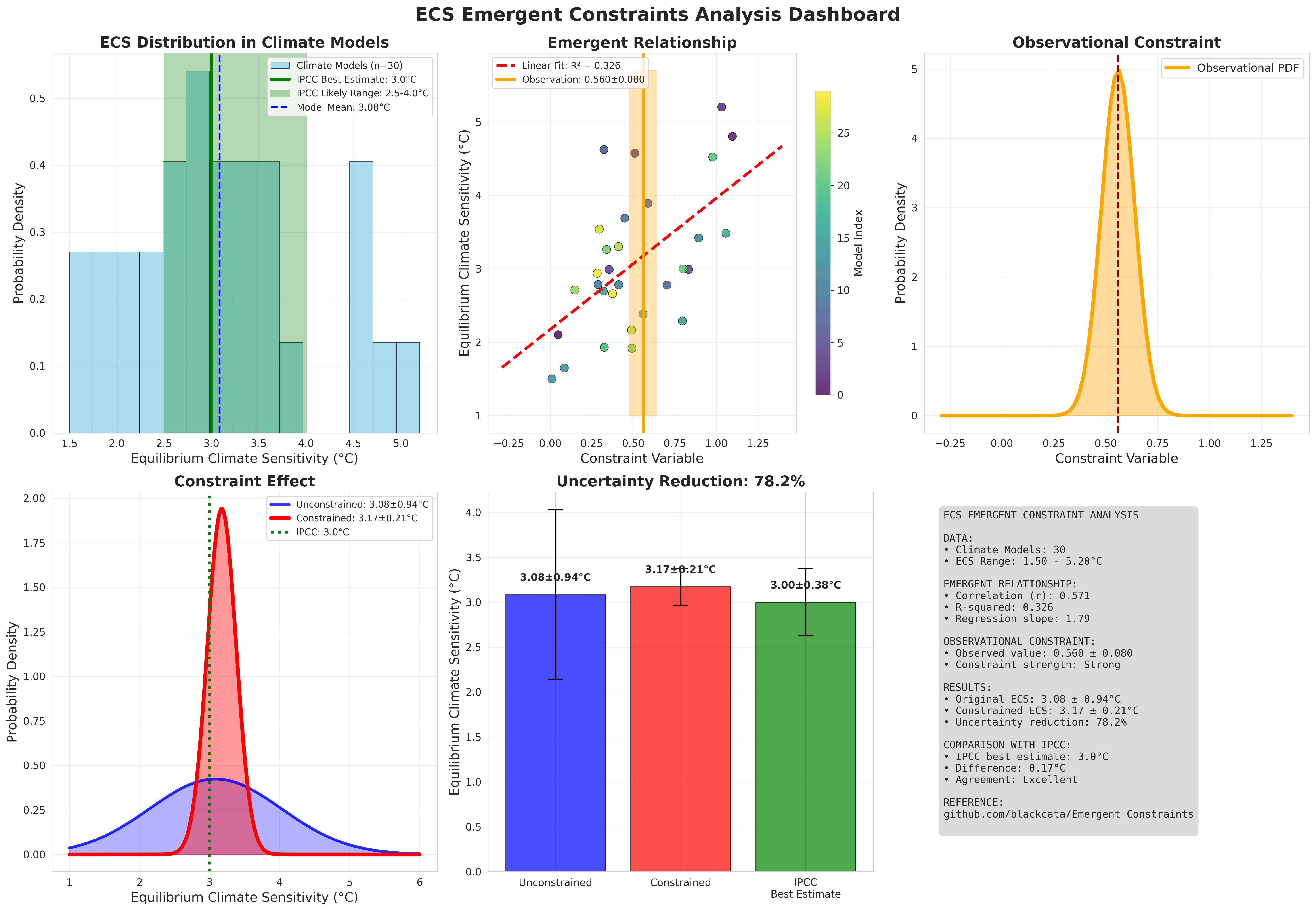
Figure 1: Complete emergent constraint analysis dashboard showing inter-model relationships, observational constraints, and uncertainty reduction.
Key Components#
Inter-model Relationship
Left Panel: Scatter plot showing the relationship between constraint variable (present-day) and target variable (future projection)
Regression Line: Linear fit through model data points
Observational Constraint: Orange vertical line with uncertainty band
Observational PDF
Center Top: Probability density function of the observational constraint
Orange Curve: Gaussian distribution representing observational uncertainty
Red Dashed Line: Mean observational value
Constraint Effect Comparison
Center Bottom: Before and after comparison of probability distributions
Blue Curve: Unconstrained (original model spread)
Red Curve: Constrained (reduced uncertainty after applying observations)
Uncertainty Reduction Statistics
Right Panel: Bar chart showing quantitative uncertainty reduction
Percentage: Shows how much the uncertainty (standard deviation) was reduced
Error Bars: Display the remaining uncertainty in each case
Method Comparison#
The emergent constraint method provides significant improvements over traditional approaches:
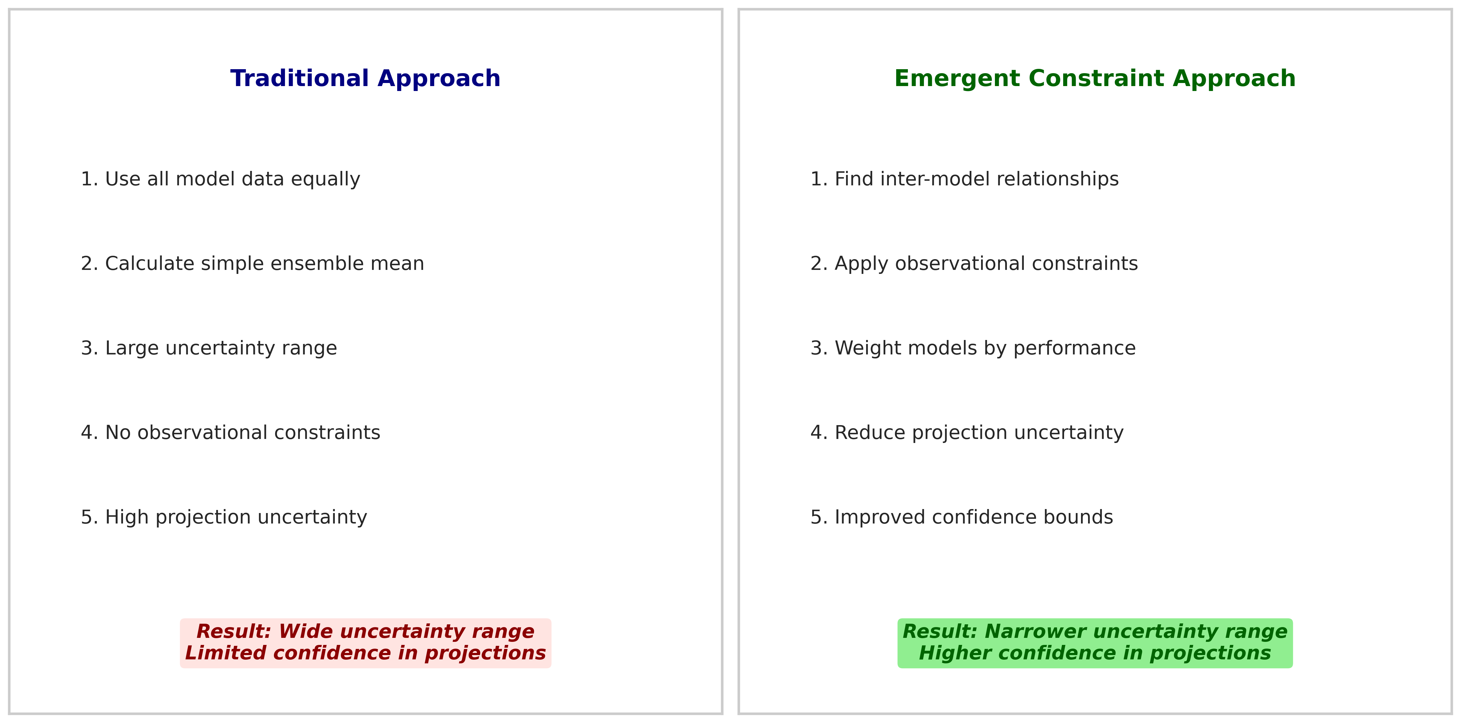
Figure 2: Comparison of traditional vs. emergent constraint methods showing uncertainty reduction.
ECS Analysis Results#
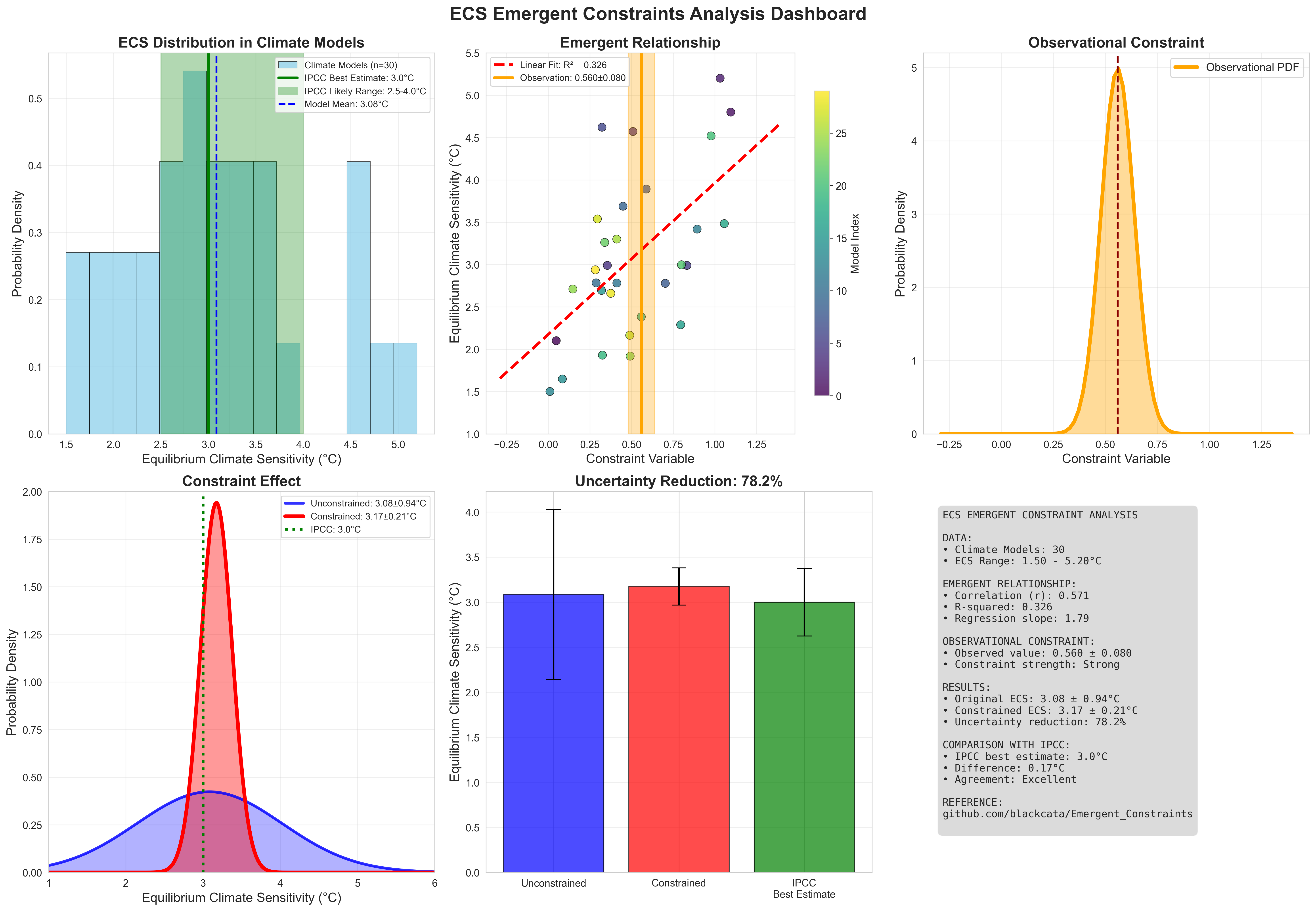
Figure 3: Detailed ECS analysis showing model distribution, constraint application, and final results.
Getting Started#
To run these analyses yourself:
Complete ECS Analysis: See Emergent Constraints Analysis for the full tutorial
GridFill Tutorial: See GridFill Tutorial: Advanced Data Interpolation for atmospheric data interpolation
Jupyter Notebook: Open
docs/source/notebooks/ecs_emergent_constraints_analysis.ipynbSimple Demo: Try
examples/emergent_constraints_demo.ipynbfor a quick start
Example Code#
import skyborn as skb
import numpy as np

# Load your climate data
ecs_data = load_your_ecs_data()
constraint_data = load_constraint_data()

# Apply emergent constraint
pdf = skb.gaussian_pdf(obs_mean, obs_std, x_grid)
correlation = skb.pearson_correlation(constraint_data, ecs_data)

# Visualize results
plot_constraint_analysis(ecs_data, constraint_data, obs_pdf)
Technical Details#
The emergent constraint method implemented in Skyborn follows established climate science practices:
Statistical Framework: Based on Bayesian inference and linear regression
Observational Integration: Incorporates measurement uncertainties
Validation: Cross-validation against independent datasets
Uncertainty Quantification: Full probabilistic treatment
Spherical Harmonic Wind Analysis (Windspharm)#
Skyborn includes a comprehensive windspharm package for spherical harmonic analysis of atmospheric wind fields. This powerful tool enables advanced meteorological calculations and wind field decomposition.
Overview#
The windspharm package provides sophisticated atmospheric analysis capabilities:
Figure 1: Fundamental atmospheric quantities - wind speed, relative vorticity, horizontal divergence, and absolute vorticity calculated using spherical harmonic analysis.
Note
Key Features:
Helmholtz Decomposition: Separates wind fields into rotational and divergent components
Vorticity & Divergence: Calculates fundamental atmospheric dynamics quantities
Streamfunction & Velocity Potential: Computes scalar representations of wind fields
Spectral Truncation: Enables filtering and smoothing of atmospheric data
Multiple Interfaces: standard and xarray interfaces for flexibility
Core Calculations#
1. Fundamental Quantities
The package calculates essential atmospheric dynamics fields:
Relative Vorticity (ζ): Measures local rotation of air parcels
Horizontal Divergence (∇·V): Quantifies expansion/contraction of flow
Absolute Vorticity: Combines relative and planetary vorticity
Wind Speed: Magnitude of horizontal wind vector
2. Helmholtz Decomposition
Separates any wind field into two fundamental components:
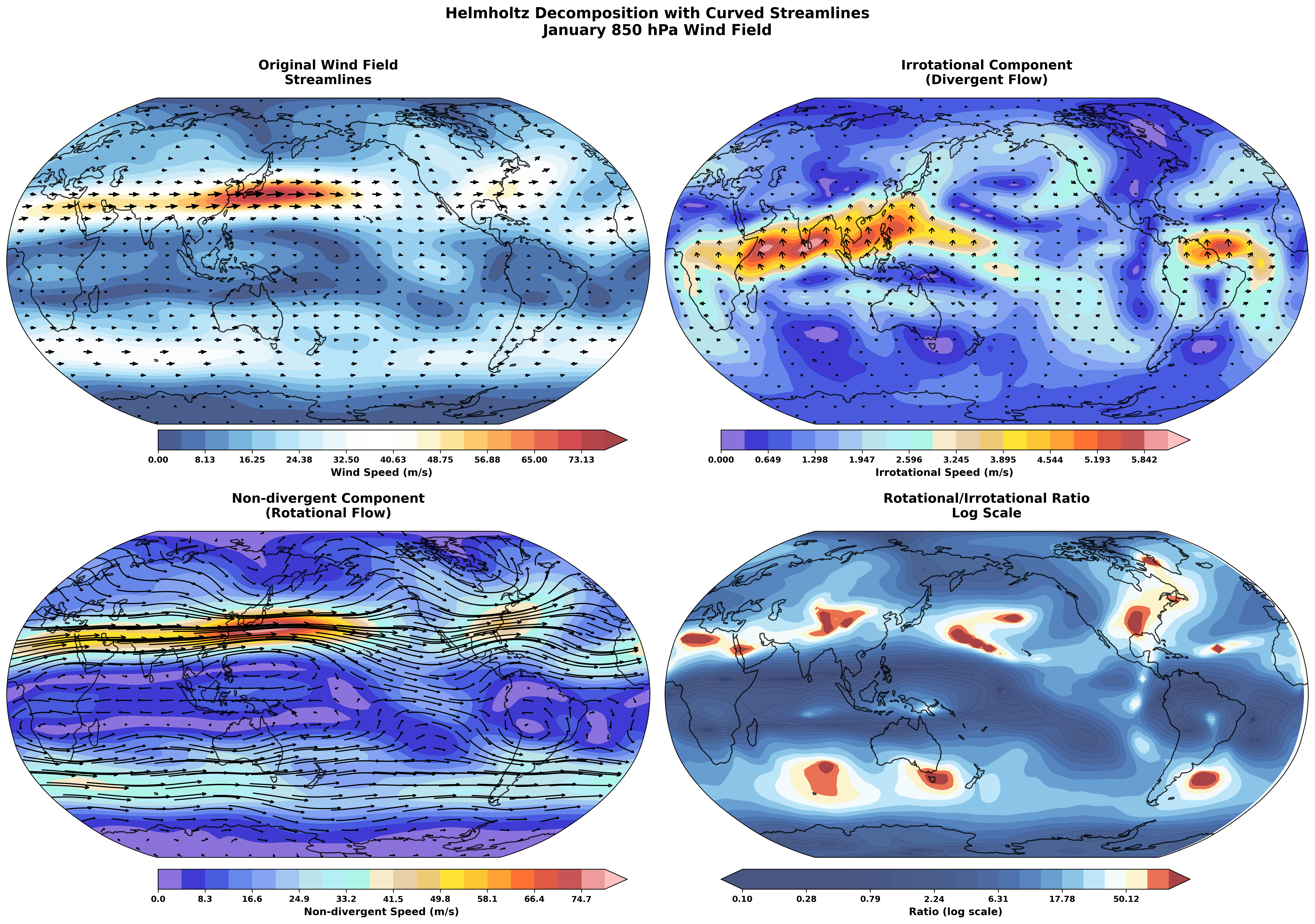
Figure 2: Helmholtz decomposition showing original wind field separated into rotational and divergent components, with streamfunction, velocity potential, and component percentages.
Rotational Component (Ψ): Non-divergent flow around low/high pressure systems
Divergent Component (χ): Irrotational flow associated with convergence/divergence
Streamfunction (Ψ): Scalar field representing rotational flow
Velocity Potential (χ): Scalar field representing divergent flow
3. Advanced Analysis
Spectral Truncation: Remove small-scale noise while preserving large-scale patterns
Planetary Vorticity: Earth’s rotation effects on atmospheric flow
Error Handling: Robust validation and coordinate checking
Performance Optimization: Efficient batch calculations for large datasets
Streamfunction and Velocity Potential Analysis#
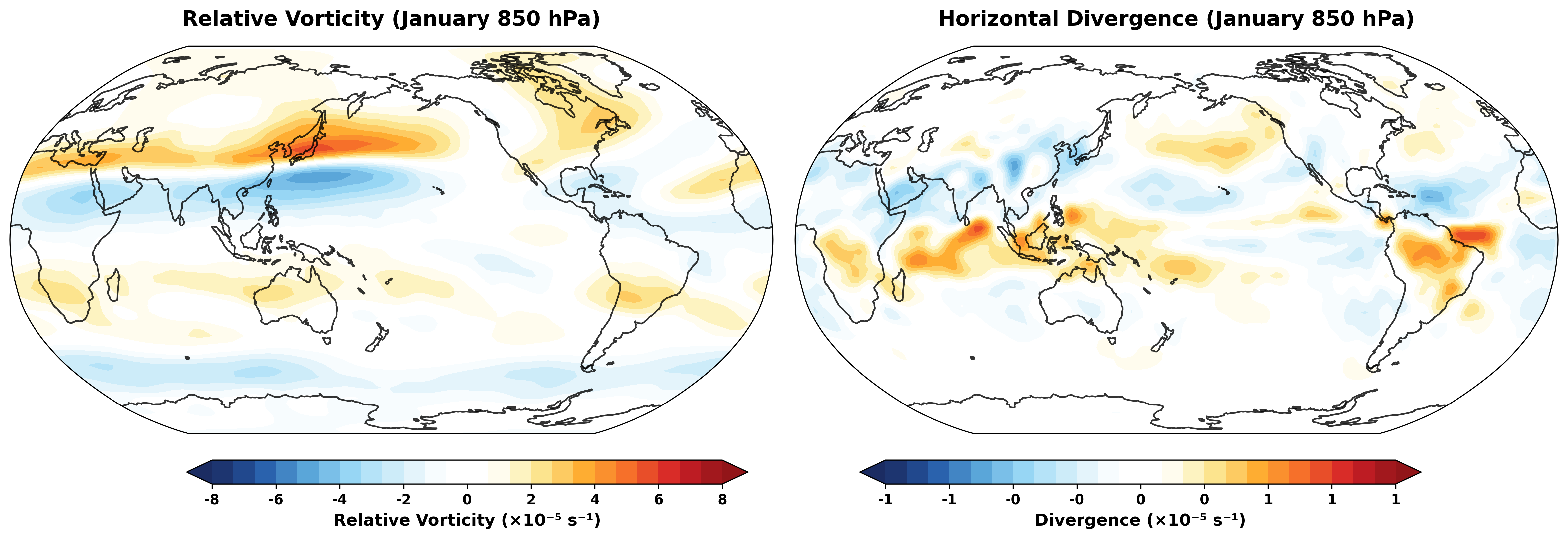
Figure 3: Detailed streamfunction and velocity potential analysis showing scalar field representations of wind flow.
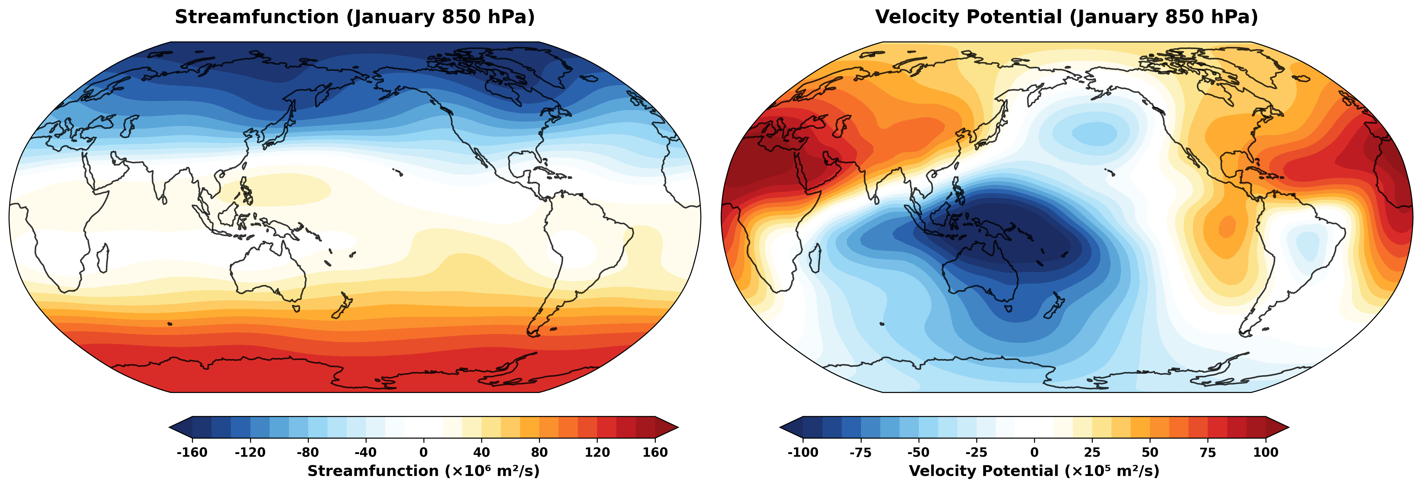
Figure 4: Comprehensive SFVP comparison demonstrating the relationship between vector and scalar wind field representations.
Component Analysis and Comparison#
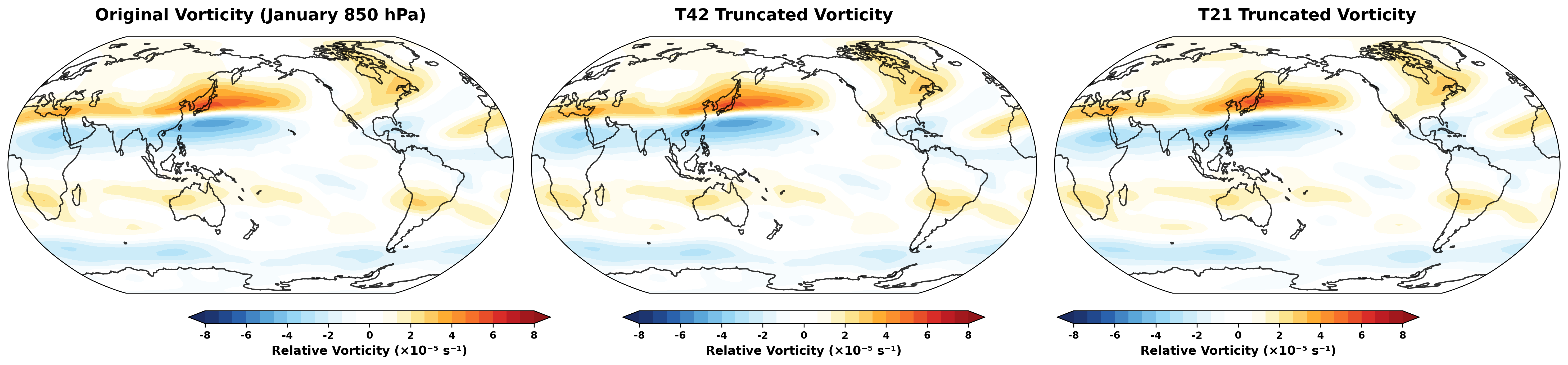
Figure 5: Component comparison analysis showing the decomposition and relationship between different wind field components.
Advanced Features#
Gradient Analysis
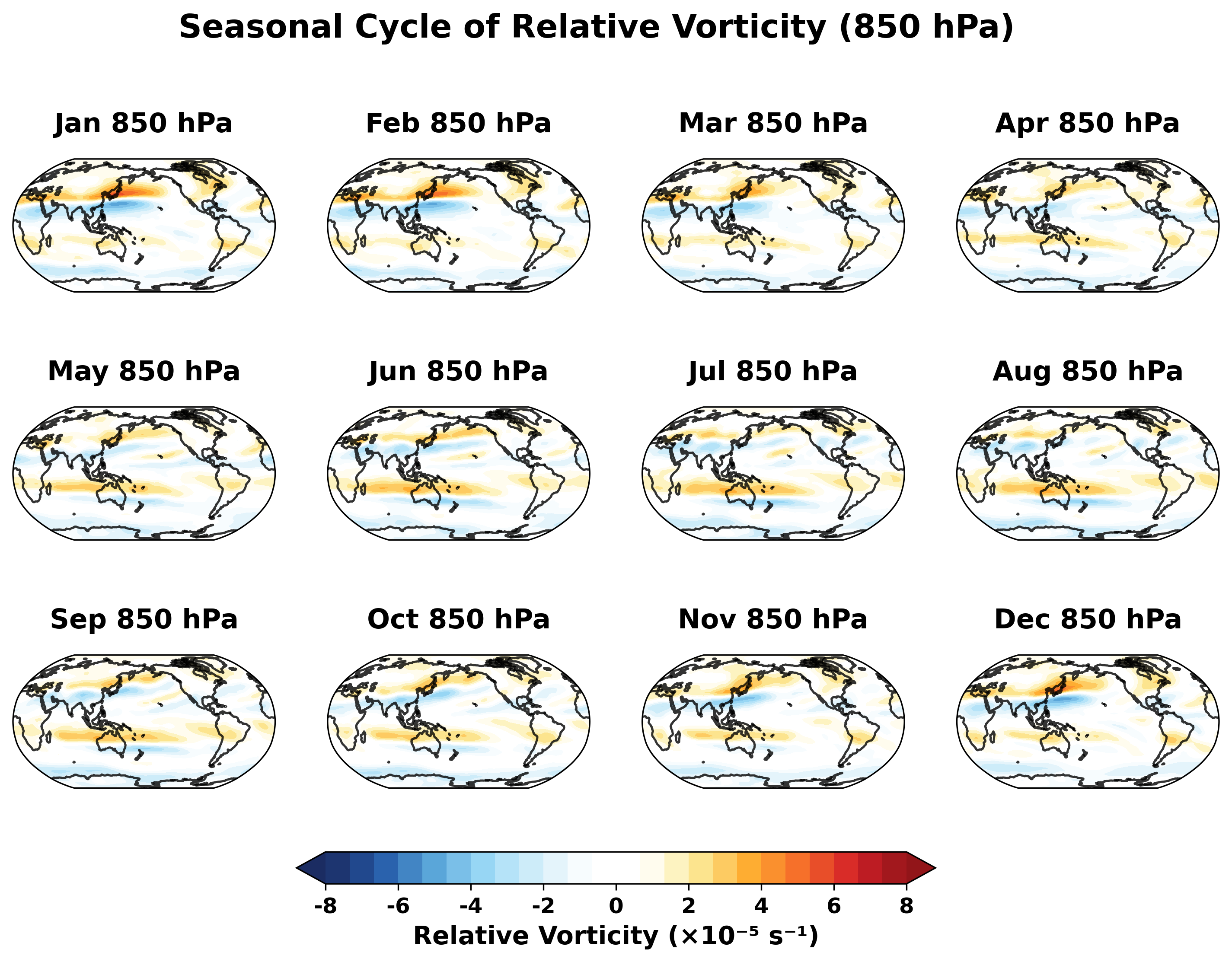
Figure 6: Gradient analysis visualization demonstrating the calculation of wind field derivatives and related quantities.
Spectral Truncation Effects
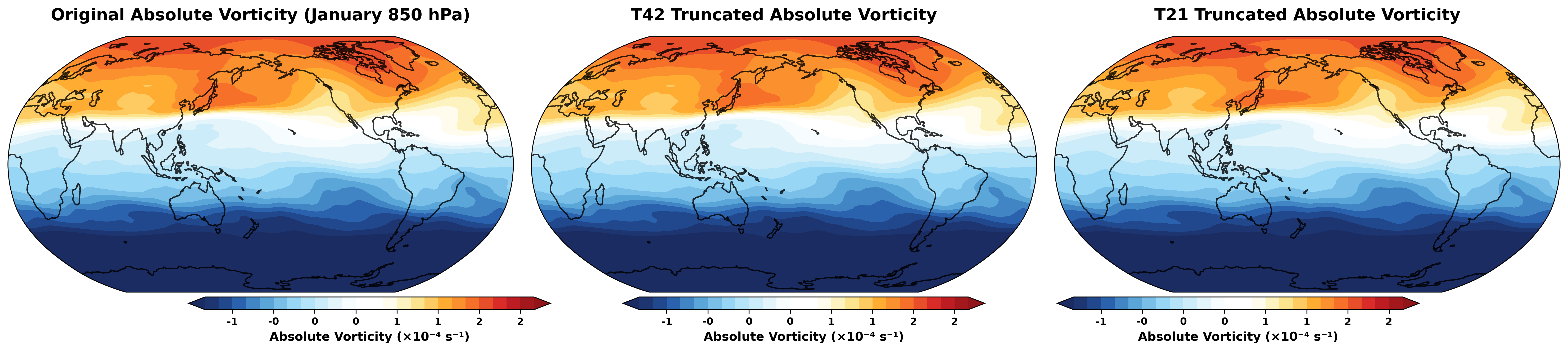
Figure 7: Spectral truncation comparison showing the effects of different truncation levels on atmospheric field analysis.
Rossby Wave Source Analysis#
Rossby Wave Source Calculation
The windspharm package includes advanced Rossby wave source analysis capabilities:
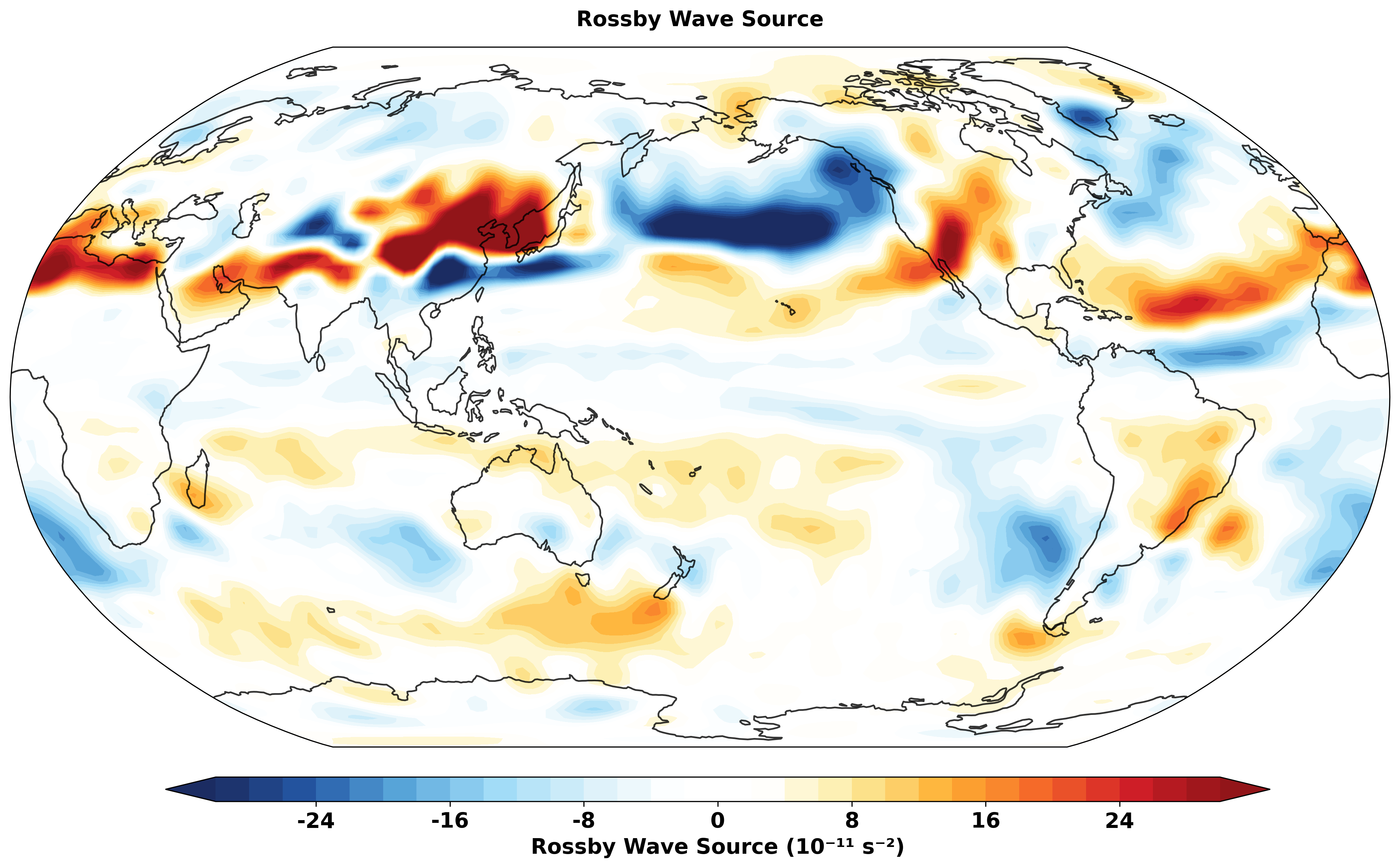
Figure 8: Rossby wave source analysis showing wave generation (red) and absorption (blue) regions. The RWS quantifies the generation of Rossby wave activity in the atmosphere.
The Rossby wave source (RWS) is calculated as:
Where: - ζₐ is absolute vorticity (relative + planetary) - ∇·v is horizontal divergence - v_χ is the irrotational (divergent) wind component - ∇ζₐ is the gradient of absolute vorticity
Physical Interpretation: - Positive RWS (Red): Rossby wave generation regions - Negative RWS (Blue): Rossby wave absorption/dissipation regions - Applications: Tropical-extratropical interactions, jet stream dynamics, storm track analysis
Truncation Effects on RWS
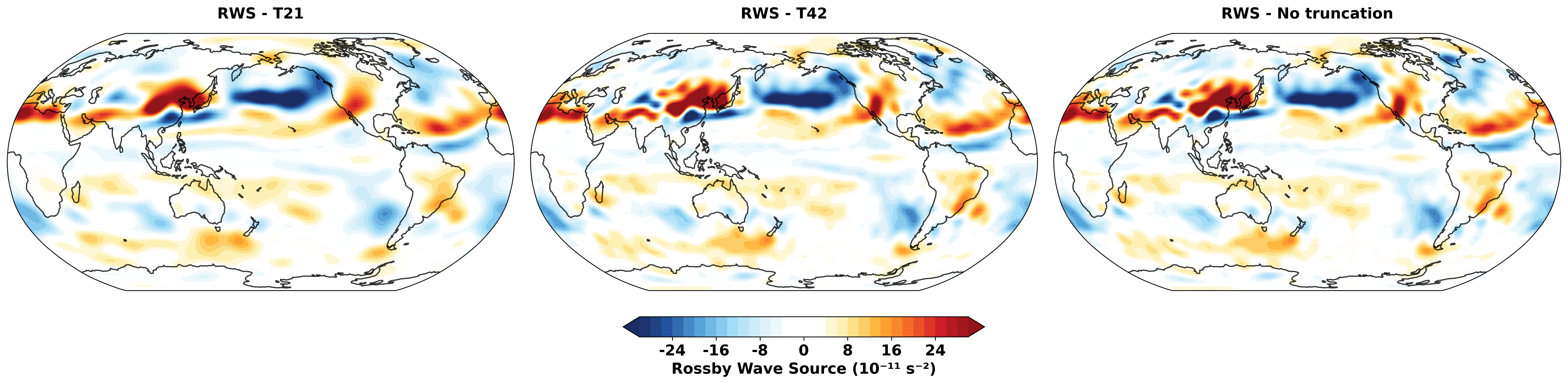
Figure 9: Comparison of Rossby wave source calculations with different spectral truncation levels (T21, T42, and no truncation) using Robinson projection and enhanced colormap.
Mathematical Foundation#
The spherical harmonic analysis is based on expanding wind fields in terms of spherical harmonics:
Where: - u, v are zonal and meridional wind components - Y_n^m are spherical harmonic functions - n, m are degree and order indices
Interactive Tutorial#
Comprehensive Tutorial: Windspharm Tutorial: Spherical Harmonic Wind Analysis
The complete windspharm tutorial demonstrates:
Data Loading: Working with NetCDF atmospheric data
Basic Calculations: Vorticity, divergence, and wind speed
Helmholtz Decomposition: Separating rotational and divergent flows
Advanced Features: Spectral truncation and performance optimization
Visualization: Creating publication-quality atmospheric plots
Best Practices: Memory management and error handling
Example Applications#
- Storm Track Analysis
Use vorticity calculations to identify and track cyclonic systems
- Jet Stream Dynamics
Apply Helmholtz decomposition to understand jet stream structure
- Rossby Wave Generation
Calculate Rossby wave source to study tropical-extratropical interactions
- Model Validation
Compare reanalysis data with climate model output using spectral methods
- Data Quality Control
Use spectral truncation to filter observational noise
Getting Started#
from skyborn.windspharm.xarray import VectorWind
import xarray as xr

# Load your wind data
ds = xr.open_dataset('Era5_Windfield_Data.nc')

# Create VectorWind object
vw = VectorWind(ds.u, ds.v)

# Calculate fundamental quantities
vorticity = vw.vorticity()
divergence = vw.divergence()

# Perform Helmholtz decomposition
uchi, vchi, upsi, vpsi = vw.helmholtz()

# Get streamfunction and velocity potential
streamfunction = vw.streamfunction()
velocity_potential = vw.velocitypotential()

# Calculate Rossby wave source
rossby_wave_source = vw.rossbywavesource()

# Analyze with different truncations
rws_t21 = vw.rossbywavesource(truncation=21)
rws_t42 = vw.rossbywavesource(truncation=42)
Technical Notes#
Grid Requirements: - Regular latitude-longitude grids - Latitude ordered north-to-south (90° to -90°) - Global coverage recommended for optimal results
Performance:
- Use batch calculations (e.g., vrtdiv()) for better performance
- Consider memory vs. speed trade-offs with legfunc parameter
- Process large datasets in chunks when memory is limited
Validation: - Built-in coordinate and data validation - Error messages guide proper usage - Reference solutions for testing
Performance Comparison#
Skyborn vs Original Windspharm Performance
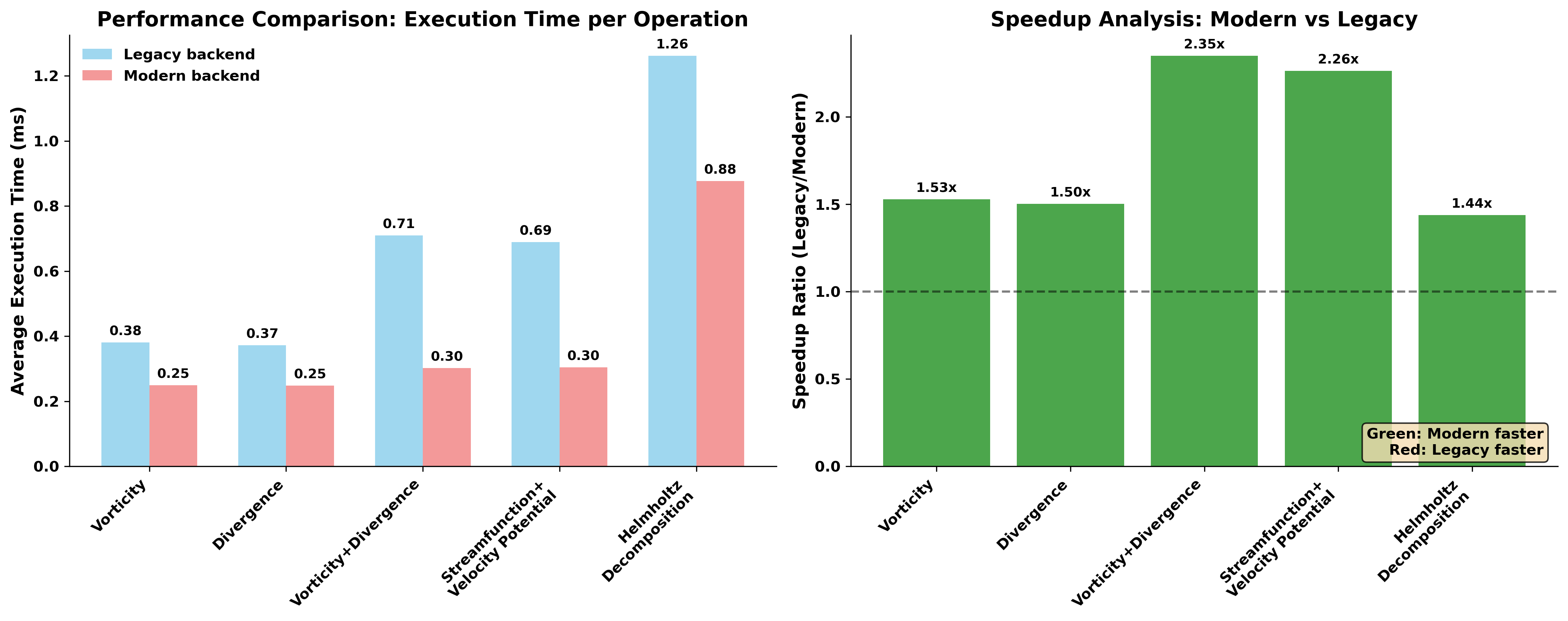
Figure 10: Performance benchmark comparison between Skyborn windspharm and original windspharm implementations. Skyborn demonstrates consistent performance improvements across all atmospheric calculations, with speedups ranging from 1.22x to 1.36x faster while maintaining identical numerical accuracy.
Key Performance Highlights:
Vorticity Calculation: 1.36x faster than original implementation
Divergence Calculation: 1.28x faster than original implementation
Combined Vorticity+Divergence: 1.25x faster than original implementation
Streamfunction+Velocity Potential: 1.31x faster than original implementation
Helmholtz Decomposition: 1.22x faster than original implementation
Numerical Accuracy: Results are identical to original windspharm
Memory Efficiency: Optimized algorithms reduce computational overhead
Consistent Performance: All operations show measurable improvements
The performance gains result from: - Optimized spherical harmonic transformations - Efficient memory management and data layout - Vectorized operations and reduced function call overhead - Algorithm optimizations specific to atmospheric wind field patterns - Enhanced caching strategies for Legendre polynomial computations
Performance Benchmarks#
Skyborn delivers exceptional performance improvements over traditional scientific computing libraries. Our optimized implementations provide significant speedups while maintaining numerical accuracy.
Statistical Analysis Performance#
Linear Regression and Mann-Kendall Trend Analysis
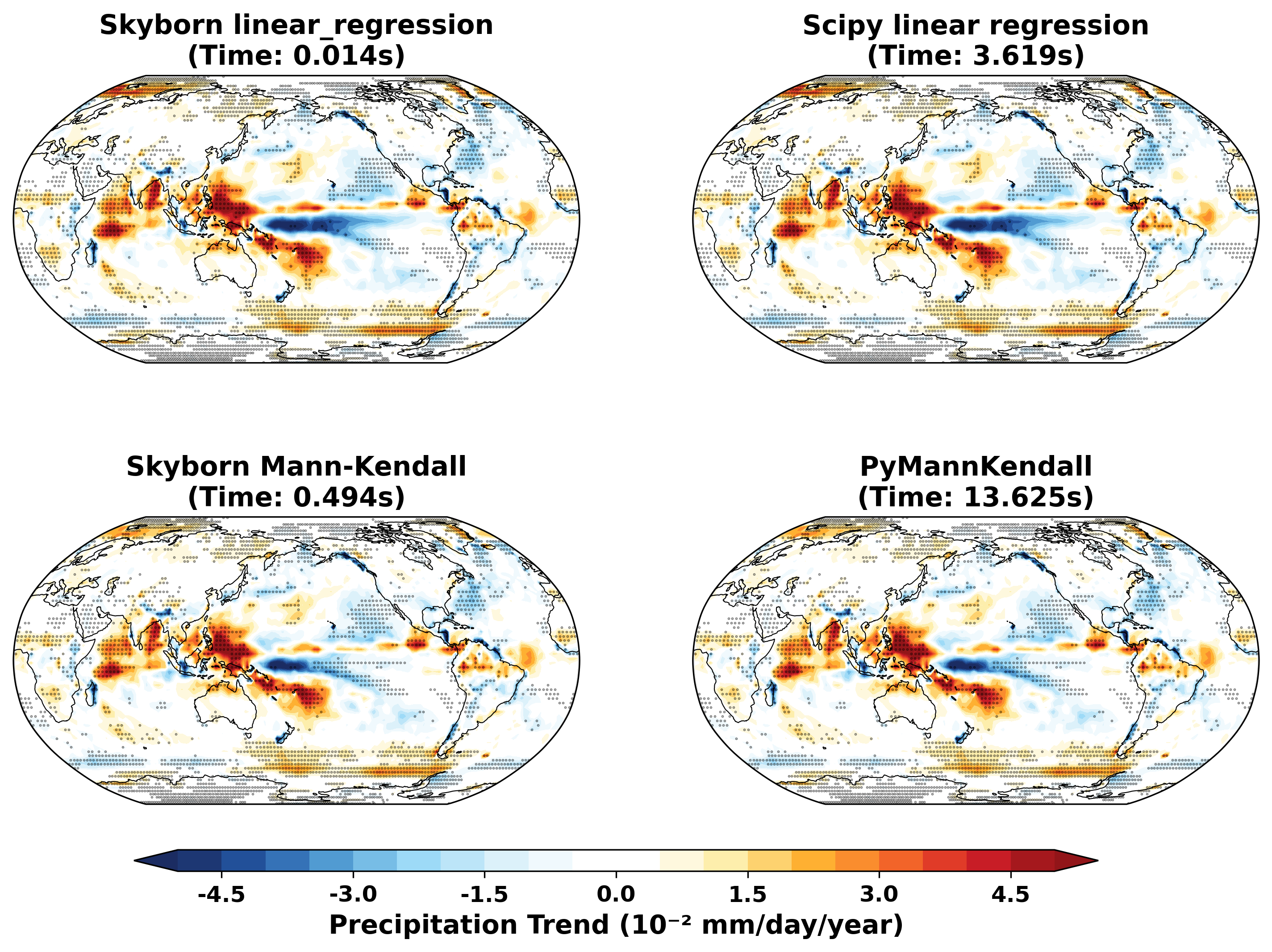
Figure 1: Performance comparison showing dramatic speed improvements: Skyborn linear regression (0.014s) vs Scipy (3.619s) - 258x faster; Skyborn Mann-Kendall (0.494s) vs PyMannKendall (13.625s) - 28x faster. Results are numerically identical between implementations.
Key Performance Highlights:
Linear Regression: 258x faster than Scipy (0.014s vs 3.619s)
Mann-Kendall Test: 28x faster than PyMannKendall (0.494s vs 13.625s)
Numerical Accuracy: Results are identical to reference implementations
Memory Efficiency: Optimized algorithms reduce memory footprint
Large Dataset Support: Performance advantages scale with data size
The performance gains come from: - Optimized NumPy operations and vectorization - Efficient memory management - Algorithm optimizations specific to climate data patterns - Reduced function call overhead - Cache-friendly data access patterns
GridFill Atmospheric Data Interpolation#
Skyborn’s GridFill module provides advanced atmospheric data interpolation capabilities using Poisson equation solvers. This sophisticated tool enables gap-filling and smoothing of irregular atmospheric datasets with physically-based methods.
Overview#
The GridFill module addresses common atmospheric data challenges:
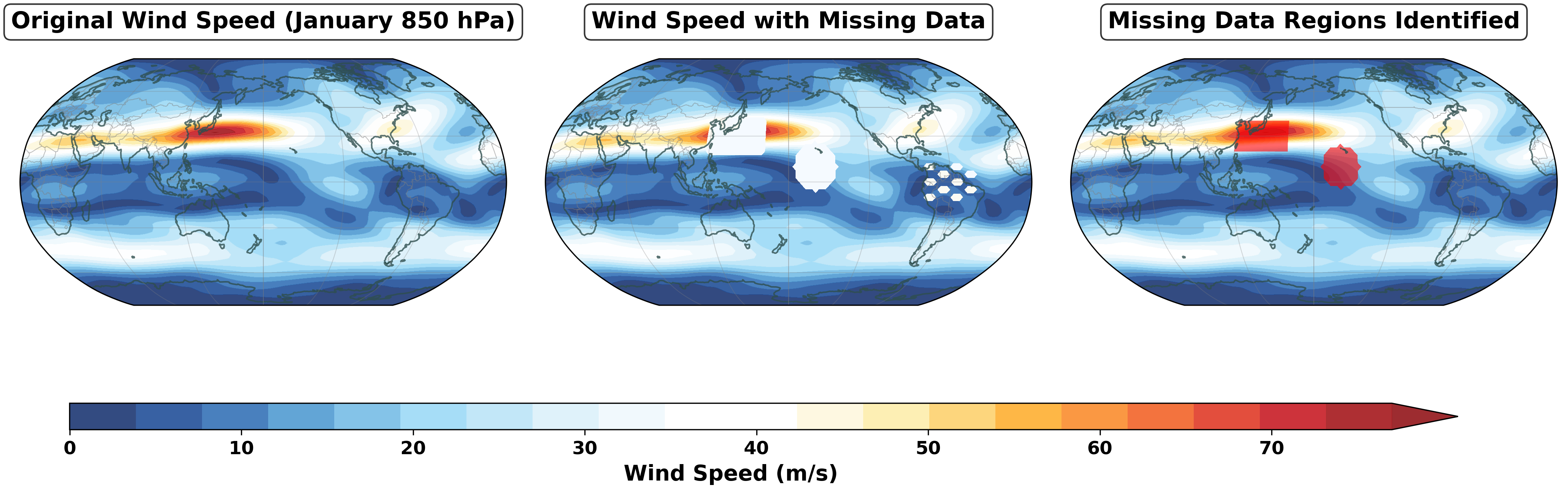
Figure 1: GridFill missing data overview showing various scenarios of missing atmospheric data patterns that require sophisticated interpolation techniques.
Note
Key Features:
Physical Basis: Solves the Poisson equation for mathematically rigorous interpolation
Multiple Interfaces: Standard, xarray, and iris compatibility for different workflows
Advanced Methods: Includes Navier-Stokes inspired formulations
Real Atmospheric Data: Optimized for meteorological and climate datasets
Gap-Filling: Efficiently handles missing data in irregular patterns
Core Functionality#
1. Basic Interpolation
The fundamental GridFill approach solves the Poisson equation:
where φ represents the atmospheric field being interpolated.
GridFill Demonstration: GPCP Precipitation Data
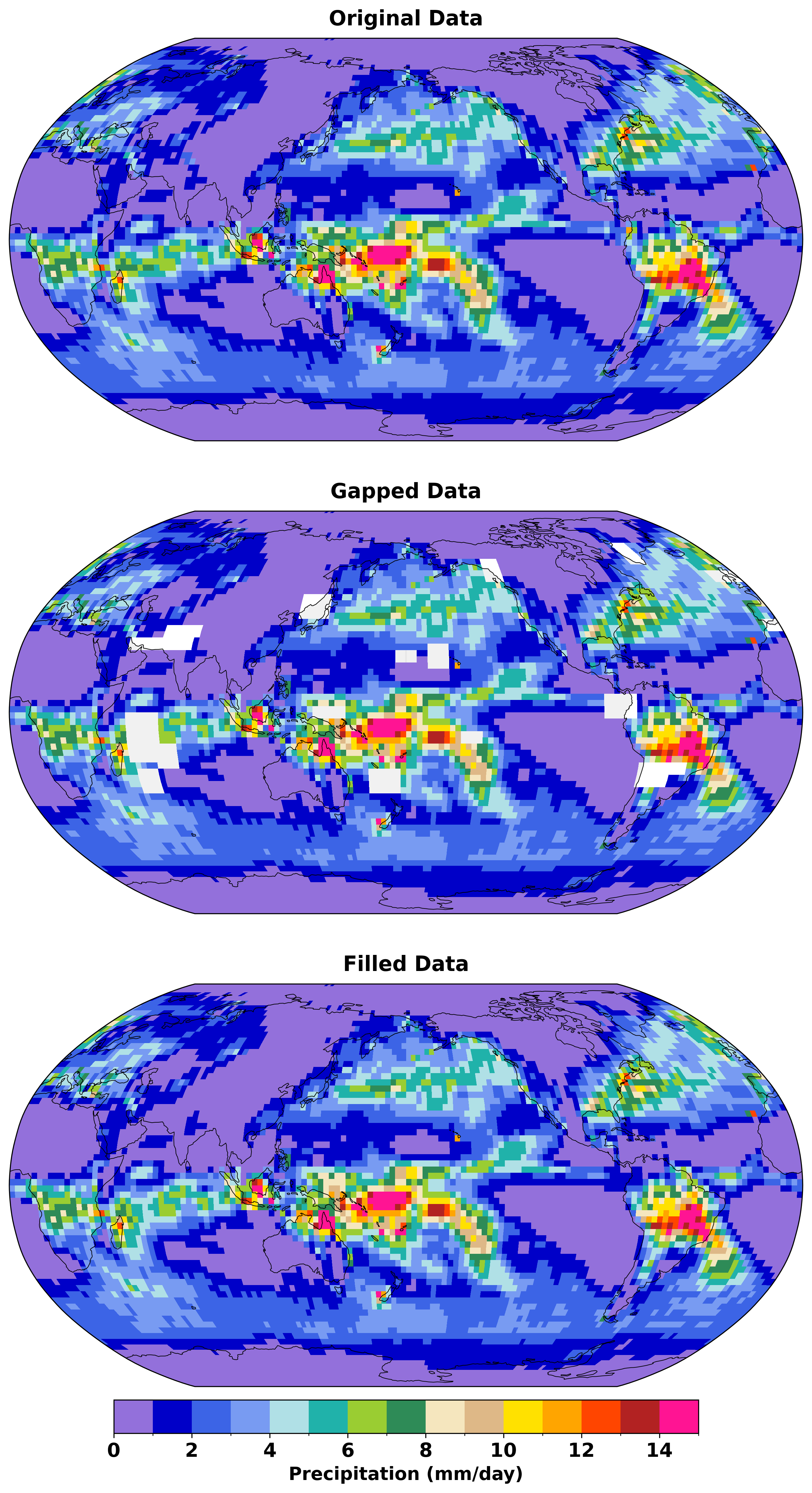
Figure: GridFill demonstration using GPCP precipitation data showing gradient-based gap placement. Top panel shows original data, middle panel shows artificially created gaps at gradient boundaries (transitions between high and low precipitation values), and bottom panel shows the filled data using Poisson equation solver. The algorithm successfully reconstructs missing values while preserving physical continuity and spatial patterns, demonstrating effectiveness at challenging interpolation scenarios.
2. Advanced Methods
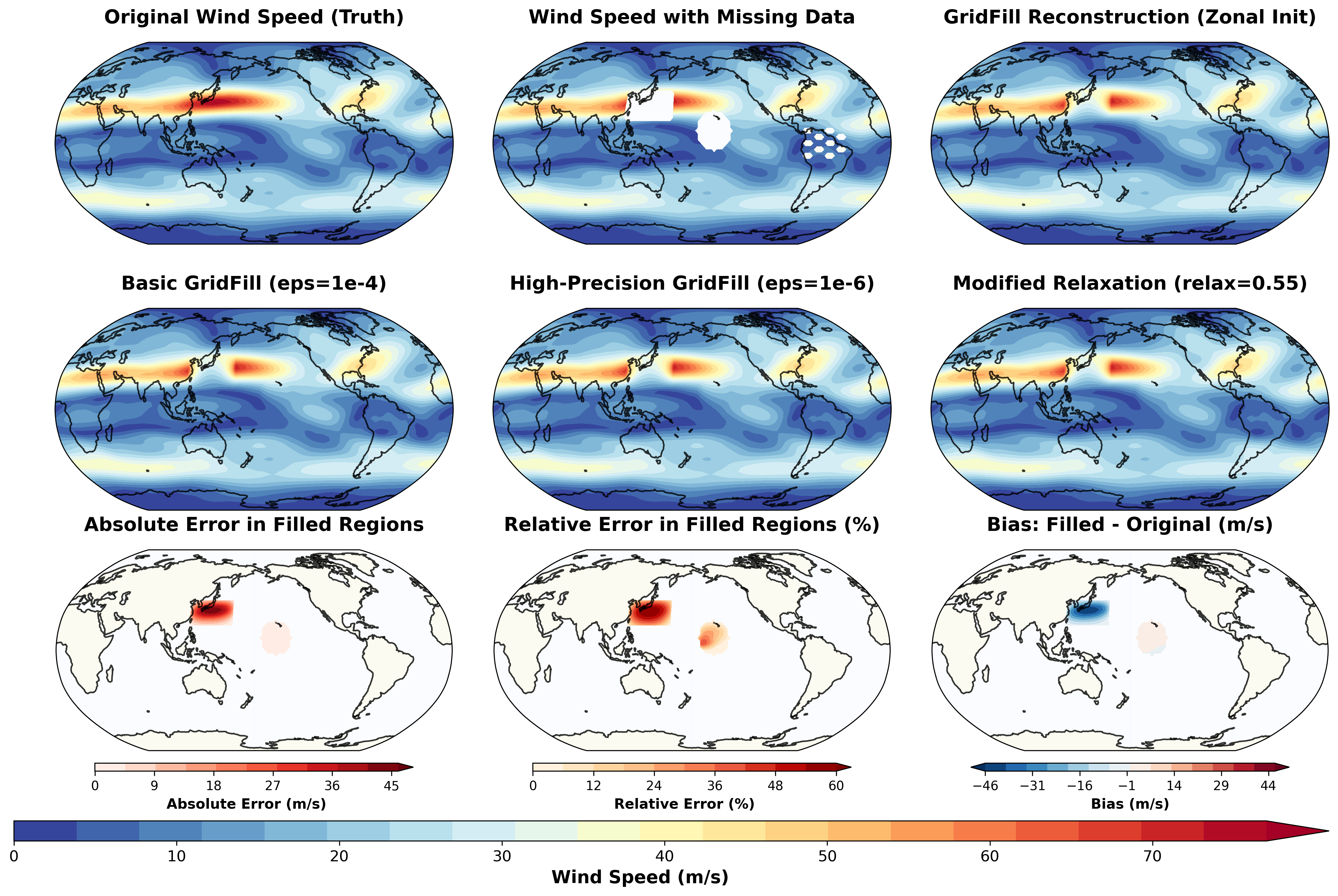
Figure 2: Comprehensive comparison of different GridFill interpolation methods showing convergence characteristics, accuracy metrics, and performance analysis across various atmospheric scenarios.
Standard GridFill: Classical Poisson equation solver
Xarray Interface: Seamless integration with modern Python climate data workflows
Iris Interface: Compatibility with the Met Office Iris library
Extended Methods: Advanced formulations for complex atmospheric phenomena
3. Quality Assessment
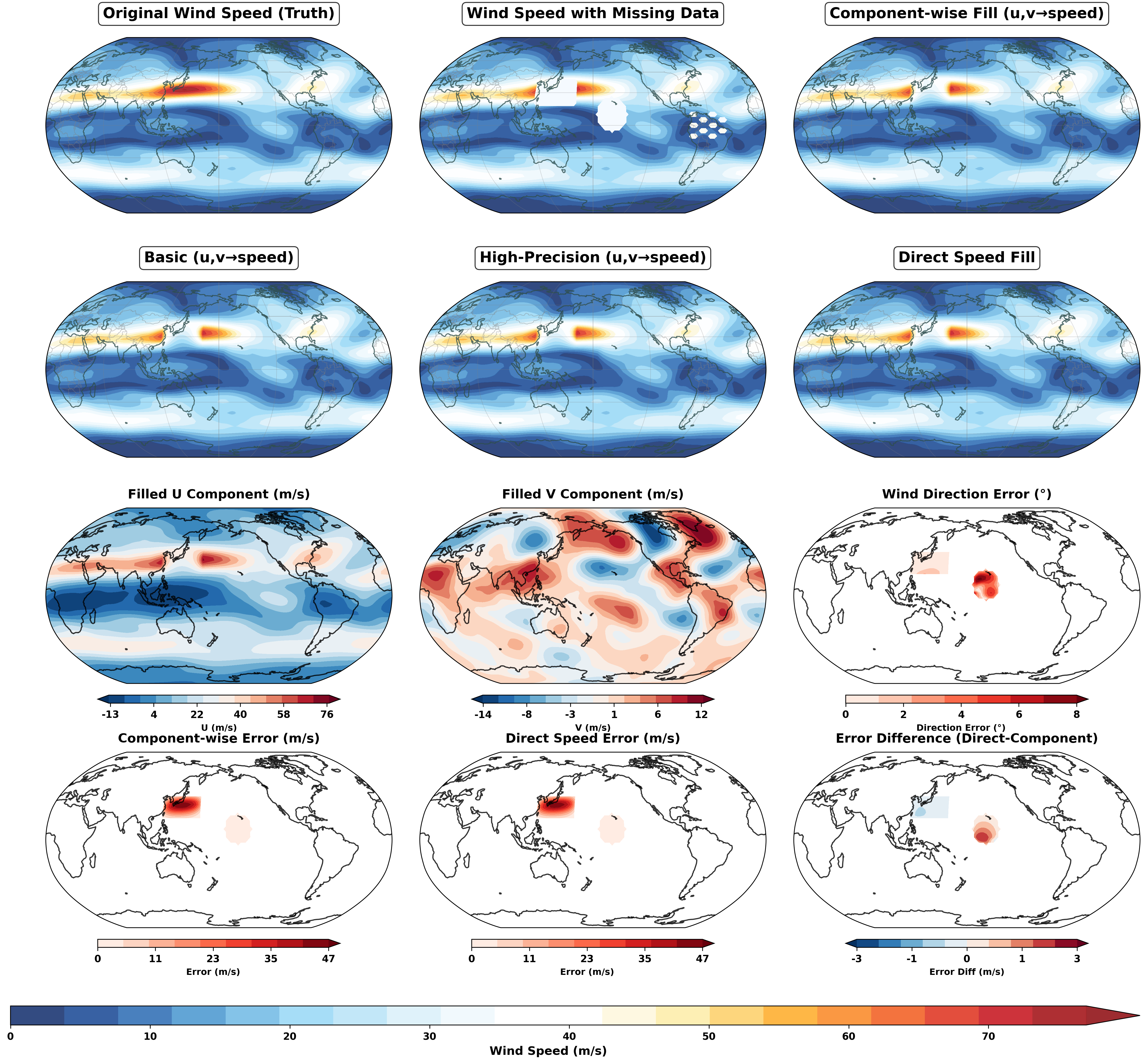
Figure 3: Component-wise vs direct approach comparison for vector wind fields, demonstrating how GridFill preserves physical constraints and maintains the integrity of atmospheric vector quantities.
Performance Analysis#
Method Comparison and Validation
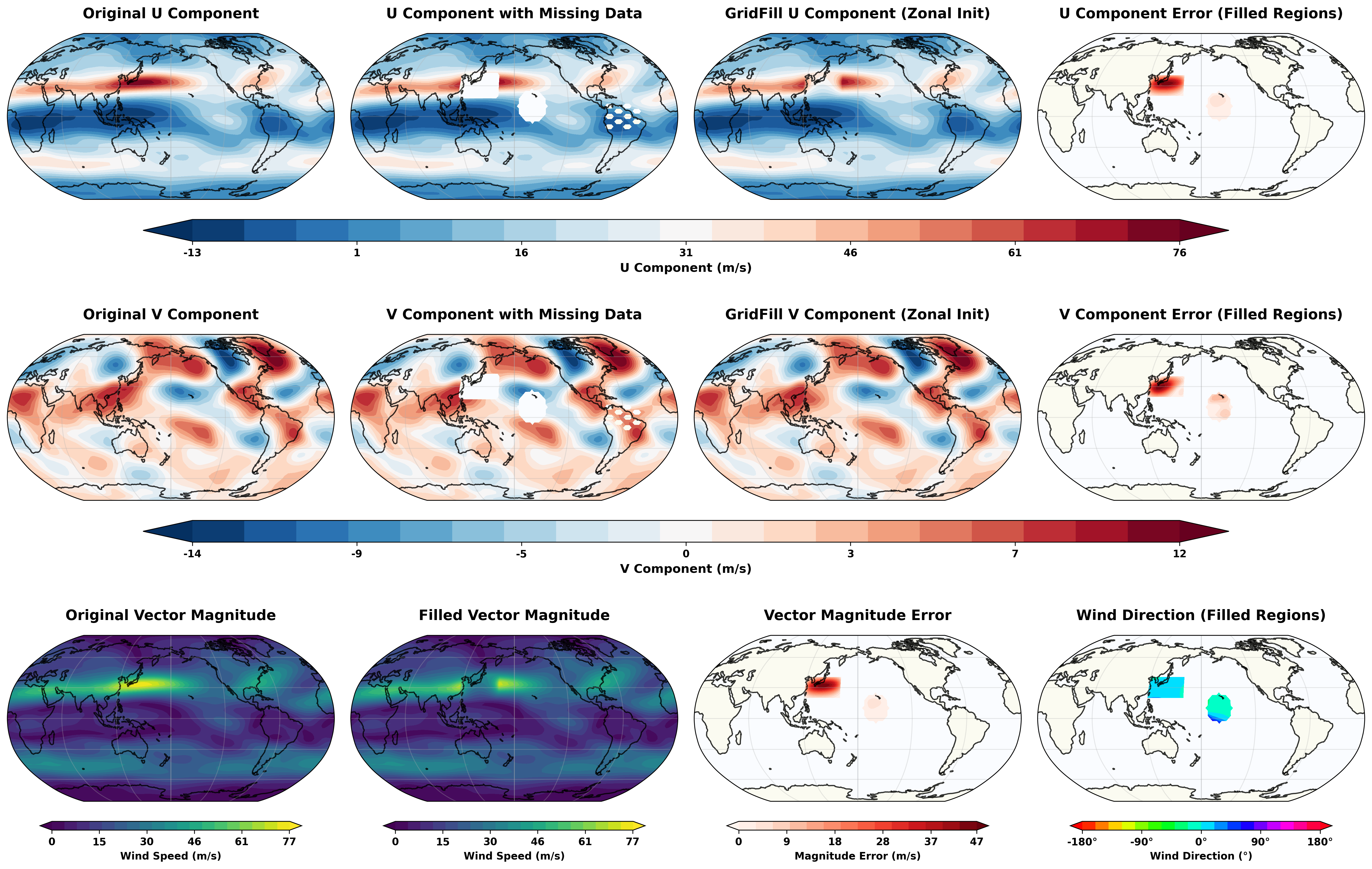
Figure 4: Detailed UV component analysis showing how GridFill handles vector wind field interpolation, preserving the physical relationships between zonal (U) and meridional (V) wind components.
The GridFill module provides robust performance across different atmospheric scenarios:
Convergence Rate: Rapid convergence for most meteorological applications
Accuracy: High precision for smooth atmospheric fields
Stability: Robust handling of irregular missing data patterns
Scalability: Efficient processing of large climate datasets
Interactive Tutorial#
Complete GridFill Tutorial: GridFill Tutorial: Advanced Data Interpolation
The comprehensive GridFill tutorial demonstrates:
Data Preparation: Loading and preprocessing atmospheric datasets
Basic Usage: Standard GridFill interface and parameters
Advanced Interfaces: Xarray and iris integration examples
Method Comparison: Quantitative analysis of different approaches
Real-World Applications: Practical atmospheric data interpolation
Performance Optimization: Tips for large dataset processing
Example Applications#
- Satellite Data Gap-Filling
Fill missing pixels in satellite-derived atmospheric products
- Station Data Interpolation
Create gridded fields from sparse observational networks
- Model Data Quality Control
Smooth numerical artifacts in climate model output
- Reanalysis Enhancement
Improve spatial coverage of atmospheric reanalysis products
- Field Campaign Support
Interpolate irregular measurement patterns from aircraft or ship data
Getting Started with GridFill#
from skyborn.gridfill.xarray import gridfill_xarray
import xarray as xr
import numpy as np

# Load atmospheric data with missing values
data = xr.open_dataset('atmospheric_data.nc')

# Create mask for missing/invalid data
mask = np.isnan(data.temperature)

# Apply GridFill interpolation
filled_data = gridfill_xarray(
    data.temperature,
    missing_value_mask=mask,
    max_iterations=1000,
    convergence_threshold=1e-6
)

# Compare original vs filled data
comparison = xr.concat([data.temperature, filled_data],
                      dim='method')
Mathematical Foundation#
GridFill implements sophisticated numerical methods:
- Poisson Equation Solver:
Iterative solution of the discrete Poisson equation with boundary conditions
- Navier-Stokes Formulation:
Advanced physics-based interpolation for fluid-like atmospheric fields
- Convergence Criteria:
Multiple stopping conditions ensure optimal balance of accuracy and efficiency
- Boundary Handling:
Sophisticated treatment of domain boundaries and irregular geometries
References#
Emergent Constraints:
Methodology: Cox, P. M., et al. (2013). Nature, 494(7437), 341-344
Implementation: Based on blackcata/Emergent_Constraints
Climate Data: CMIP5/CMIP6 model ensembles
IPCC Assessment: AR6 Working Group I Report
Spherical Harmonics:
Mathematical Foundation: Spherical harmonic expansion theory
Key References: Swarztrauber, P. N. (2000). Generalized Discrete Spherical Harmonic Transforms. Journal of Computational Physics 213-230.
Implementation: Based on established meteorological practices
Validation: Cross-verified against reference implementations
GridFill Interpolation:
Mathematical Foundation: Poisson equation solver for atmospheric data gap-filling
Implementation: Based on the gridfill package by Andrew Dawson (ajdawson/gridfill)
Numerical Methods: Finite difference relaxation schemes for 2D Poisson equation (∇²φ = 0)
Atmospheric Applications: Optimized for meteorological and oceanographic data interpolation
Boundary Conditions: Support for cyclic (global) and non-cyclic (regional) grids
- Key References:
Numerical methods for partial differential equations in atmospheric sciences
Finite difference methods for fluid dynamics applications
Climate data quality control and gap-filling techniques