Tutorial: Mann-Kendall Trend Analysis with Real GPCP Precipitation#

Audience:

Users who want to compare Skyborn against loop-based regression and Mann-Kendall baselines on a real global precipitation dataset.

Prerequisites:

Local GPCP monthly precipitation file at GPCP.precip.mon.mean.nc
cartopy, scipy, pymannkendall, and cmaps available in the active environment

Learning goals:

Load and prepare a real monthly precipitation dataset from GPCP
Benchmark four common trend-analysis workflows on annual means
Compare multiple Mann-Kendall test families on the same precipitation field
Visualize significance masks with skyborn.plot.scatter

Outline#

Setup and load the real GPCP dataset
Build annual-mean precipitation for 1979-2014
Benchmark four methods with the same 2D layout
Compare additional Mann-Kendall test families on annual GPCP trends
Compare seasonal Mann-Kendall families on monthly GPCP data

from __future__ import annotations

from pathlib import Path
import time
import warnings

import cartopy.crs as ccrs
import cartopy.feature as cfeature
import cmaps
import matplotlib.pyplot as plt
import numpy as np
import pymannkendall as pmk
import xarray as xr
from scipy import stats

from skyborn.calc import linear_regression, mann_kendall_multidim, mann_kendall_xarray
from skyborn.plot import scatter

DATA_PATH = Path(r"GPCP.precip.mon.mean.nc")
FIGURE_DIR = Path(r"../images")
FIGURE_DIR.mkdir(parents=True, exist_ok=True)

if not DATA_PATH.exists():
    raise FileNotFoundError(
        f"GPCP file not found: {DATA_PATH}. Update DATA_PATH before running this notebook."
    )

warnings.filterwarnings("ignore", category=RuntimeWarning, message="invalid value encountered in sqrt")
plt.rcParams["figure.dpi"] = 140
plt.rcParams["savefig.dpi"] = 140
plt.rcParams["axes.titlesize"] = 11
plt.rcParams["axes.labelsize"] = 10

TREND_SCALE = 100.0
TREND_MAX = 5.0
LEVELS = np.linspace(-TREND_MAX, TREND_MAX, 21)
CMAP = cmaps.BlueWhiteOrangeRed
NORM = plt.Normalize(vmin=-TREND_MAX, vmax=TREND_MAX)
SIG_LEVEL = 0.05

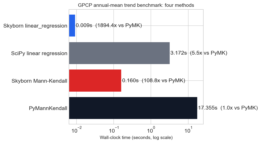
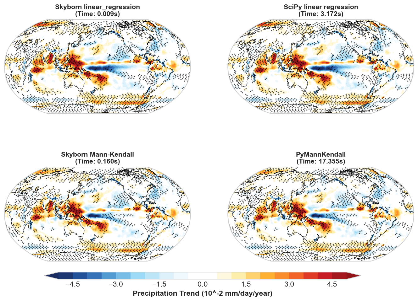
Step 2 - Benchmark four methods on the same annual field#

This section keeps the same layout you were already using:

Skyborn linear_regression
SciPy stats.linregress loop
Skyborn mann_kendall_multidim(..., test="original")
pymannkendall.original_test loop

All four methods use the same annual GPCP field and the same significance threshold.

def benchmark_four_methods(pr_annual: xr.DataArray) -> dict[str, object]:
    pr = pr_annual.values.astype(np.float64)
    year = pr_annual["year"].values.astype(np.float64)
    lat = pr_annual["lat"].values
    lon = pr_annual["lon"].values

    start_time = time.perf_counter()
    pr_trend_skyborn, p_values_skyborn = linear_regression(pr, year)
    time_skyborn = time.perf_counter() - start_time

    pr_trend_scipy = np.full((len(lat), len(lon)), np.nan, dtype=np.float64)
    p_values_scipy = np.full((len(lat), len(lon)), np.nan, dtype=np.float64)
    start_time = time.perf_counter()
    for i in range(len(lat)):
        for j in range(len(lon)):
            series = pr[:, i, j]
            if np.isfinite(series).all():
                slope, intercept, r_value, p_value, std_err = stats.linregress(year, series)
                pr_trend_scipy[i, j] = slope
                p_values_scipy[i, j] = p_value
    time_scipy = time.perf_counter() - start_time

    start_time = time.perf_counter()
    mk_result = mann_kendall_multidim(pr, axis=0, test="original", method="theilslopes")
    time_mk_skyborn = time.perf_counter() - start_time
    pr_trend_mk_skyborn = mk_result["trend"]
    p_values_mk_skyborn = mk_result["p"]

    pr_trend_pmk = np.full((len(lat), len(lon)), np.nan, dtype=np.float64)
    p_values_pmk = np.full((len(lat), len(lon)), np.nan, dtype=np.float64)
    start_time = time.perf_counter()
    for i in range(len(lat)):
        for j in range(len(lon)):
            series = pr[:, i, j]
            if np.isfinite(series).all():
                result = pmk.original_test(series)
                pr_trend_pmk[i, j] = result.slope
                p_values_pmk[i, j] = result.p
    time_pmk = time.perf_counter() - start_time

    return {
        "lat": lat,
        "lon": lon,
        "timings": {
            "Skyborn linear_regression": time_skyborn,
            "SciPy linear regression": time_scipy,
            "Skyborn Mann-Kendall": time_mk_skyborn,
            "PyMannKendall": time_pmk,
        },
        "fields": {
            "Skyborn linear_regression": {
                "trend": pr_trend_skyborn * TREND_SCALE,
                "p": p_values_skyborn,
            },
            "SciPy linear regression": {
                "trend": pr_trend_scipy * TREND_SCALE,
                "p": p_values_scipy,
            },
            "Skyborn Mann-Kendall": {
                "trend": pr_trend_mk_skyborn * TREND_SCALE,
                "p": p_values_mk_skyborn,
            },
            "PyMannKendall": {
                "trend": pr_trend_pmk * TREND_SCALE,
                "p": p_values_pmk,
            },
        },
        "consistency": {
            "linear_trend_max_abs": float(np.nanmax(np.abs(pr_trend_skyborn - pr_trend_scipy))),
            "linear_p_max_abs": float(np.nanmax(np.abs(p_values_skyborn - p_values_scipy))),
            "mk_trend_max_abs": float(np.nanmax(np.abs(pr_trend_mk_skyborn - pr_trend_pmk))),
            "mk_p_max_abs": float(np.nanmax(np.abs(p_values_mk_skyborn - p_values_pmk))),
        },
    }


def plot_trend_panel(ax, lon, lat, trend, p_values, title):
    ax.set_global()
    ax.add_feature(cfeature.COASTLINE, linewidth=0.5)
    ax.add_feature(cfeature.OCEAN, color="lightgray", alpha=0.5)
    im = ax.contourf(
        lon,
        lat,
        trend,
        levels=LEVELS,
        cmap=CMAP,
        norm=NORM,
        transform=ccrs.PlateCarree(),
        extend="both",
    )
    scatter(
        ax,
        lon,
        lat,
        where=np.isfinite(p_values) & (p_values < SIG_LEVEL),
        density=2.0,
        s=1,
        c="black",
        alpha=0.55,
        transform=ccrs.PlateCarree(),
    )
    ax.set_title(title, fontweight="bold")
    return im


benchmark = benchmark_four_methods(pr_annual)
benchmark["timings"], benchmark["consistency"]

({'Skyborn linear_regression': 0.009161099995253608,
  'SciPy linear regression': 3.171522399992682,
  'Skyborn Mann-Kendall': 0.15956569999980275,
  'PyMannKendall': 17.354746500001056},
 {'linear_trend_max_abs': 3.755242644620793e-15,
  'linear_p_max_abs': 2.2426505097428162e-14,
  'mk_trend_max_abs': 1.3877787807814457e-17,
  'mk_p_max_abs': 0.0})

labels = list(benchmark["timings"].keys())
times = np.array(list(benchmark["timings"].values()), dtype=float)
speedup_vs_pmk = benchmark["timings"]["PyMannKendall"] / times

fig, ax = plt.subplots(figsize=(8, 4.5))
bar_colors = ["#2563eb", "#6b7280", "#dc2626", "#111827"]
bars = ax.barh(labels, times, color=bar_colors)
ax.set_xscale("log")
ax.set_xlabel("Wall-clock time (seconds, log scale)")
ax.set_title("GPCP annual-mean trend benchmark: four methods")
ax.invert_yaxis()
for bar, t, s in zip(bars, times, speedup_vs_pmk):
    ax.text(t * 1.05, bar.get_y() + bar.get_height() / 2, f"{t:.3f}s  ({s:.1f}x vs PyMK)", va="center")
plt.tight_layout()
plt.show()

../_images/b317a8e777d7d36ab81289499142be224616ef4345492e880733228f1092a194.png

lon = benchmark["lon"]
lat = benchmark["lat"]

fig = plt.figure(figsize=(12, 8))

ax1 = plt.subplot(2, 2, 1, projection=ccrs.Robinson(central_longitude=180))
im1 = plot_trend_panel(
    ax1,
    lon,
    lat,
    benchmark["fields"]["Skyborn linear_regression"]["trend"],
    benchmark["fields"]["Skyborn linear_regression"]["p"],
    f"Skyborn linear_regression\n(Time: {benchmark['timings']['Skyborn linear_regression']:.3f}s)",
)

ax2 = plt.subplot(2, 2, 2, projection=ccrs.Robinson(central_longitude=180))
plot_trend_panel(
    ax2,
    lon,
    lat,
    benchmark["fields"]["SciPy linear regression"]["trend"],
    benchmark["fields"]["SciPy linear regression"]["p"],
    f"SciPy linear regression\n(Time: {benchmark['timings']['SciPy linear regression']:.3f}s)",
)

ax3 = plt.subplot(2, 2, 3, projection=ccrs.Robinson(central_longitude=180))
plot_trend_panel(
    ax3,
    lon,
    lat,
    benchmark["fields"]["Skyborn Mann-Kendall"]["trend"],
    benchmark["fields"]["Skyborn Mann-Kendall"]["p"],
    f"Skyborn Mann-Kendall\n(Time: {benchmark['timings']['Skyborn Mann-Kendall']:.3f}s)",
)

ax4 = plt.subplot(2, 2, 4, projection=ccrs.Robinson(central_longitude=180))
plot_trend_panel(
    ax4,
    lon,
    lat,
    benchmark["fields"]["PyMannKendall"]["trend"],
    benchmark["fields"]["PyMannKendall"]["p"],
    f"PyMannKendall\n(Time: {benchmark['timings']['PyMannKendall']:.3f}s)",
)

cbar_ax = fig.add_axes([0.2, 0.1, 0.6, 0.02])
cbar = plt.colorbar(im1, cax=cbar_ax, orientation="horizontal", extend="both")
cbar.set_label("Precipitation Trend (10^-2 mm/day/year)", fontweight="bold", fontsize=12)
plt.show()

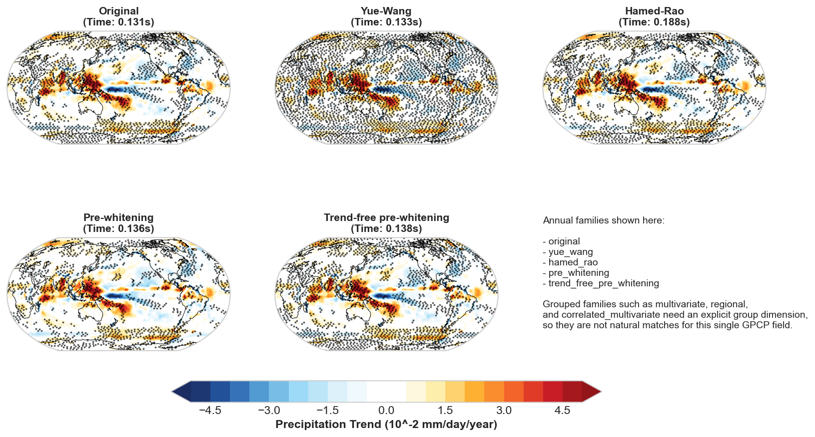
../_images/268fa124e674d3dc3df29033078f7b97c82e0b316c072adebfbc42b3b0d896d9.png

Step 3 - Additional annual Mann-Kendall test families#

The next figure switches away from the four-method benchmark and focuses only on Skyborn’s Mann-Kendall family support. These annual tests all use the same annual GPCP field, but they differ in how they handle serial correlation before estimating significance.

annual_test_labels = {
    "original": "Original",
    "yue_wang": "Yue-Wang",
    "hamed_rao": "Hamed-Rao",
    "pre_whitening": "Pre-whitening",
    "trend_free_pre_whitening": "Trend-free pre-whitening",
}

annual_family_results = {}
for test_name in annual_test_labels:
    start_time = time.perf_counter()
    result = mann_kendall_xarray(pr_annual, dim="year", test=test_name, use_dask=False)
    annual_family_results[test_name] = {
        "result": result,
        "elapsed": time.perf_counter() - start_time,
    }

{
    key: {
        "time_s": round(value["elapsed"], 3),
        "trend_mean": float(value["result"]["trend"].mean().values),
        "p_mean": float(value["result"]["p"].mean().values),
    }
    for key, value in annual_family_results.items()
}

{'original': {'time_s': 0.131,
  'trend_mean': 0.0005843882468302479,
  'p_mean': 0.30874893760779976},
 'yue_wang': {'time_s': 0.133,
  'trend_mean': 0.0005843882468302479,
  'p_mean': 0.14570934915756303},
 'hamed_rao': {'time_s': 0.188,
  'trend_mean': 0.0005843882468302479,
  'p_mean': 0.301690559168806},
 'pre_whitening': {'time_s': 0.136,
  'trend_mean': 0.0005843882468302479,
  'p_mean': 0.3460342612478936},
 'trend_free_pre_whitening': {'time_s': 0.138,
  'trend_mean': 0.0005843882468302479,
  'p_mean': 0.3026199075317609}}

fig = plt.figure(figsize=(14, 8))
for idx, (test_name, label) in enumerate(annual_test_labels.items(), start=1):
    ax = plt.subplot(2, 3, idx, projection=ccrs.Robinson(central_longitude=180))
    ds = annual_family_results[test_name]["result"]
    im = plot_trend_panel(
        ax,
        ds["lon"].values,
        ds["lat"].values,
        ds["trend"].values * TREND_SCALE,
        ds["p"].values,
        f"{label}\n(Time: {annual_family_results[test_name]['elapsed']:.3f}s)",
    )

ax_note = plt.subplot(2, 3, 6)
ax_note.axis("off")
ax_note.text(
    0.0,
    0.95,
    """Annual families shown here:

- original
- yue_wang
- hamed_rao
- pre_whitening
- trend_free_pre_whitening

Grouped families such as multivariate, regional,
and correlated_multivariate need an explicit group dimension,
so they are not natural matches for this single GPCP field.""",
    va="top",
    fontsize=10,
)

cbar = fig.colorbar(im, ax=fig.axes[:5], orientation="horizontal", fraction=0.05, pad=0.07, extend="both")
cbar.set_label("Precipitation Trend (10^-2 mm/day/year)", fontweight="bold", fontsize=12)
plt.show()

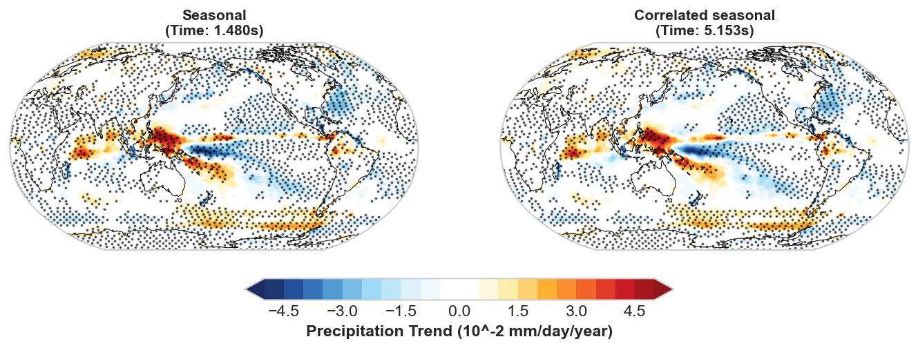
../_images/b6a0d8a0a8cff97778a7c38e3ad178a5495eaf2d82b4d611b7d6913a56066d58.png

Step 4 - Seasonal Mann-Kendall families on monthly GPCP data#

Seasonal families should stay on the monthly series and use period=12. This keeps the full seasonal cycle instead of collapsing it into annual means first.

seasonal_test_labels = {
    "seasonal": "Seasonal",
    "correlated_seasonal": "Correlated seasonal",
}

seasonal_family_results = {}
for test_name in seasonal_test_labels:
    start_time = time.perf_counter()
    result = mann_kendall_xarray(
        pr_monthly,
        dim="time",
        test=test_name,
        period=12,
        use_dask=False,
    )
    seasonal_family_results[test_name] = {
        "result": result,
        "elapsed": time.perf_counter() - start_time,
    }

{
    key: {
        "time_s": round(value["elapsed"], 3),
        "trend_mean": float(value["result"]["trend"].mean().values),
        "p_mean": float(value["result"]["p"].mean().values),
    }
    for key, value in seasonal_family_results.items()
}

{'seasonal': {'time_s': 1.48,
  'trend_mean': -0.001439065561152902,
  'p_mean': 0.22914402255009053},
 'correlated_seasonal': {'time_s': 5.153,
  'trend_mean': -0.001439065561152902,
  'p_mean': 0.27210238420612737}}

fig = plt.figure(figsize=(12, 4.8))
for idx, (test_name, label) in enumerate(seasonal_test_labels.items(), start=1):
    ax = plt.subplot(1, 2, idx, projection=ccrs.Robinson(central_longitude=180))
    ds = seasonal_family_results[test_name]["result"]
    im = plot_trend_panel(
        ax,
        ds["lon"].values,
        ds["lat"].values,
        ds["trend"].values * TREND_SCALE,
        ds["p"].values,
        f"{label}\n(Time: {seasonal_family_results[test_name]['elapsed']:.3f}s)",
    )

cbar = fig.colorbar(im, ax=fig.axes, orientation="horizontal", fraction=0.06, pad=0.08, extend="both")
cbar.set_label("Precipitation Trend (10^-2 mm/day/year)", fontweight="bold", fontsize=12)
plt.show()

../_images/4812d4e0086d4301420e9638a169e3cf19064c8de8a3af2eeabbec7ea03499f5.png

Notes#

The four-method benchmark intentionally keeps two loop-based baselines so the speed difference is visible on the same real field.
The annual MK family figure uses annual means from 1979-2014.
The seasonal MK family figure keeps the monthly data and uses period=12.
All significance masks are plotted with skyborn.plot.scatter rather than Axes.scatter, so the retained stipple density responds to the displayed map geometry.

Tutorial: Mann-Kendall Trend Analysis with Real GPCP Precipitation

Contents